Numerical Investigation of 2D Lid Driven Cavity using
Smoothed Particle Hydrodynamics (SPH) Method
C. S. Nor Azwadi
a, Z. Mohamad Shukri
band M. Y. Afiq Witri
aa
Faculty of Mechanical Engineering,Universiti Teknologi Malaysia, 81310 Skudai, Johor Bahru
b
Faculty of Mechanical Engineering,Universiti Teknikal Malaysia Melaka, 76100 Durian Tunggal, Melaka
Abstract. This paper describes the formulation of fluid equation in application of Smoothed Particle Hydrodynamics (SPH) and ability of meshfree SPH method to model lid driven cavity problem. Although the lid driven cavity problem are usually successfully solved using traditional Finite Difference Method (FDM), they are all depends on the mesh ability. This SPH method is relatively new approach in solving fluid flow problem. The SPH method can be used to discretize the Navier–Stokes equation that governs fluid flows. In the present study, the ability of the meshless SPH method are investigate in simulating the fluid flow which is in 2D lid driven cavity problem. The result of this problem using meshfree SPH method is compare to the solution done using meshing software Fluent with Reynold Number 1 and it shows that the SPH method give good comparison to the FDM method.
Keywords: PACS:
INTRODUCTION
Simulation of incompressible flows is very important topic in computational fluid dynamics (CFD). Traditionally grid-based numerical methods such as finite element method (FEM), finite difference method (FDM) and finite volume method (FVM) are used to simulate incompressible flows. FEM, FDM and FVM have been dominating the field of CFD for quite a long period of time. Recently growing interests have been focused on the meshless methods or meshfree methods as alternatives for traditional grid-based methods. Meshfree method is developed which successfully avoid the process of regenerating the whole mesh in the large deformation scenario. One of the meshfree methods is smoothed particle hydrodynamics (SPH) method which can solve problem without meshing process. The objective in the present work is to develop and document a numerical tool to determine the velocity field in the 2D lid driven cavity using SPH formulation.
SPH BACKGROUND
Smooth Particle Hydrodynamics (SPH) is meshfree, pure Lagrangian particle method for modeling fluid flow which is originally developed for simulating astrophysics phenomena. There are many particle methods but these notes are concerned with Smoothed Particle Hydrodynamics (SPH) devised by Gingold and Monaghan [1] and by Lucy [2].
SPH FORMULATION
There are two steps in using SPH method which is Kernel approximation and particle approximation. Both steps are presented in the next section.
Basic Concept
The SPH method is based on the interpolation theory. The method allows any function to be expressed in terms of its values at a set of disordered points, the particles. If we consider A(x) as a typical field variable at a certain position, x, in space, the kernel approximation of A(x) is defined as [1]
(
a)
s(
a)
(
a b, )
'
A x
o
A x W x
x h dx
(1)where h represents the smoothing length and W is a weighting function with the following properties
(
a b, )
1
space
W x
x h dr
³
(2)0
lim
W x
(
ax h
b, )
(
x
ax
b)
o
w
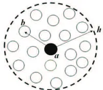
(3)This continuous integral representation of kernel approximation Equation 1 can be converted to discretized form of summation over all the particles in the support domain as shown in Figure 1.
FIGURE 1. Particle approximation within support domain for particle a. The support domain is circular with a radius of smoothing length, h.
Eventually, Equation 1 can be expressed in following Equation 3 for particle approximation form;
(
)
b b
a b a b b ab
b b b b
A
A
A
m
W
m
W
U
U
¦
x
x
¦
(4)where Wab known as kernel function of particle a. For its derivative, change are made only on the it’s kernel
function
b
a b ab
b b
A
A
m
W
U
¦
(5)Alternatively, for symmetric and less sensitive to particle disordered Equation 5 can be rewrite as follows
1
a b b a ab
b a
A
m
A
A
W
U
Kernel Function
Kernel function is the most important part of the SPH method. Various forms of kernels with different compact support have been proposed by many researchers. The stability of the SPH algorithm depends strongly upon the second derivative of the kernel. In this work, cubic spline kernel was used. If defining Rab= xab/h = (xb - xa)/h, the
cubic spline function can be written as
2 3
3
2
1
; 0
1
3
2
1
( , )
(2
)
; 1
2
6
0
;
2
ab d
R
R
R
W R h
W
R
R
R
D
d d
°
°
°
d d
®
°
d
°
°¯
(7)where Įd = 1/h and 15/7h2 corresponding to one and two dimensional spaces respectively.
MATHEMATICAL MODELLING
By assuming the fluids are isothermal, the Navier Stokes equations can be used in a simplified form. Fluid is expressed by a velocity field v, a density field ȡ and a pressure field p. Thus by expressing the evolution of the fluid in the time, we get an equation for conservation of mass and conservation of momentum [6].
Conservation of mass
The governing equations of conservation of mass for incompressible flows in Lagrange form can be written as follows
d
.
d
t
U
U
v
(8)For incompressible flow, there is no change in density, Thus Equation 8 become
.
0
U
v
(9)Apply the SPH particle approximation identity from Equation 6 into Equation 9,
(
)
b(
)
0
a a a b a a ab
b b
m
W
U
U
U
v
¦
v
v
(10)Where pa is density of particle a. The symmetric form would be
(
)
b(
)
(
)
0
a a a b a a ab b b a a ab
b a b
m
W
m
W
U
U
U
v
¦
v
v
¦
v
v
(11)Conservation of momentum
Time rate of change of the velocity (momentum equation) define as
2
v
v
v
g
p
t
U
ª
«
w
x
º
»
U
P
w
¬
¼
v
(12)Since the particle itself represents the mass, the conservation of mass is guarantee. Using following identity
0
v
x
v
(13)Thus yield for single particle a and neglecting the effect of gravity, g, Equation 12 become
2
.
a
a a
d
P
dt
U
P
U
§
·
§ ·
¨
¸
¨ ¸
©
¹
©
¹
v
v
(14)
Apply the SPH particle approximation identity from Equation 4 on the first term (pressure) and second term (viscosity) on the RHS of Equation 14.Thus yield
b
b a ab
b a b
a
P
P
m
W
U
U U
§
·
¨
¸
©
¹
¦
(15)2 2
.
b ab ab
b a b
v
v
m
w
P
P
U
U U
§ ·
¨ ¸
© ¹
¦
v
(16)
The problem with Equations 15 on the pressure term above is that the forces resulting are not necessarily symmetric. When we compute this force for two particles which don’t have the same pressure or velocity, the forces are different, and the third Newton’s law is violated. Many approaches exist to make this equation symmetric. This paper will use approach from [3].
2 2
b a
b a ab
b b a
a
P
P
P
m
W
U
U
U
§
·
§
·
¨
¸
¨
¸
©
¹
¦
©
¹
(17)By combination of Equation 16 and Equation 17, then Equation 14 become
2 2 2
a b a b a
b a ab b ab
b b a b a b
d
P
P
v
v
m
W
m
w
dt
U
U
P
U U
§
·
¨
¸
©
¹
¦
¦
v
(18)State Equation
In order to update the quantities of the particles, we need to know the pressure p. Pressure can be compute using following state of equation for incompressible flows of water and low Reynolds number
2
P
c
U
(19)Apply SPH particle approximation from Equation 4, the density at particle a, ȡa may be evaluate using
b
a b ab b ab
b b b
m
W
m W
U
U
U
¦
¦
(20)Time Integration
A modified Euler technique was used to perform the time integration. For stability, several time step criteria must be satisfied and subjected to CFL condition. Morris et. al. [5] suggested the expression for estimating time step when considering viscous diffusion are
2
0.125
h
t
X
' d
(21)where h is smoothing length and is kinetic viscosity
The leapfrog method is used for its low requirement on memory storage and its computational efficiency. In the leapfrog method, the particle velocities and positions are offset by a half time step when integrating the equations of motion. At the end of the first time step (t0), the change in density and velocity are used to advance the density and velocity at half a time step, while the particle positions are advanced in a full time step.[1]
0 2 2/ 2
/ 2
.
/ 2
t
i o i o i
t
i o i o i
i o i o i o
t
t
t
t
t
t
D
t
t
v t
t
v t
Dv t
t
x t
t
x t
t v t
t
U
U
'U
'
'
'
'
'
'
'
'
'
(22)In order to keep the calculations consistent at each subsequent time step, at the start of each subsequent time step, the density and velocity of each particle need to be predicted at half a time step to coincide the position.
2 2/ 2
/ 2
ti i i
t
i i i
t
t
t
D
t
t
v t
v t
t
Dv t
t
U
U
'U
'
'
'
'
'
(23)At the end of the subsequent time step, the particle density, velocity and position are advanced in the standard leapfrog scheme
/ 2
/ 2
..
/ 2
/ 2
..
.
/ 2
i i i
i o i i
i i i o
t
t
t
t
t
t
t
t D
t
v t
t
v t
t
t Dv t
x t
t
x t
t v t
t
U
U
U
'
'
'
'
'
'
'
'
'
'
(24)
Figure 2 shows the solution procedure that we employed in this paper.
Initializing
FIGURE 2. Solution procedure
NUMERICAL SETUP
In this section, the initial conditions and simulation steps are explained. The lid-driven cavity problem is a flow within a closed square with the topside moving at a constant velocity, while the other three sides stay stationary. The flow will reach an equilibrium state, which behaves in a recirculation pattern. The flow is sketched on Figure 3.
FIGURE 3. The considered flow. The lid is moving with a constant velocity Utop.
In this SPH simulation, the dimension of the side of the square domain is l = 1x10⁻³ meter. The top side of the squares moves at the velocity of Utop = 1x10⁻³m/s. The kinetic viscosity are and density are = 1x10⁻⁶ m/s2 and ȡ = 1x10³ kg/m3 respectively. This corresponding to Reynolds Number of 1 using
Neighbor Particle Search
Smoothing Function Calculation
Calculating Internal, External, and Viscous force Density Calculation
Update position, velocity, etc.. Calculate momentum change rate
[image:6.595.220.391.557.665.2]Re
U l
topX
(25)The sound speed was taken as c = 0.01 m/s correspond to Mach numbers of M = 0.1. A total of 40× 40 = 1600 SPH real particles are initially placed in the square region. A constant time step of 5 x 10⁻⁵ s was used. It takes approximately 3000 steps to reach a steady state which is approximately 0.15 seconds.
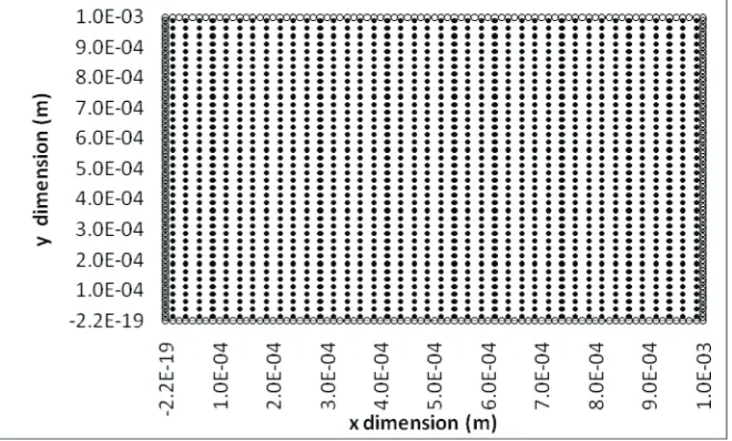
The implementation of boundary condition are done with introducing the virtual particle or called ghost particle [4]. In this 2D lid cavity problem, 80 virtual boundary particles were placed surrounding the geometry of the square cavity. Which is will produce 320 virtual particle. The 80 boundary virtual particle on top side of cavity will setting to the velocity of 1x10⁻³ m/s while the other virtual particle located on 3 other side are set to be 0 m/s. This boundary virtual particle will exerting the repulsive force which is will bounce back the real particle when collide with them. The distribution of this boundary particle and real particle are shown in Figure 4.
Results were compared with the simulation done on the same problem by using software Fluent with discretization of the momentum of equation done by applying Finite Different Method of Second Order Upwind Scheme. For consistency purpose, the simulation on Fluent is done by using 40x40 grid mesh.
RESULTS AND DISCUSSIONS
The initial distribution of particle before simulating is shown in Figure 4, while Figure 5 shows the actual particle position after steady state (0.15 seconds).This plot shows that SPH produce the expected physics of the problem.
FIGURE 4. Initial distribution of 1600 (40 x 40) real particle (filled circle) within equally space in square cavity and 320 virtual boundary particle (unfilled circle) were placed surrounding of the square cavity.
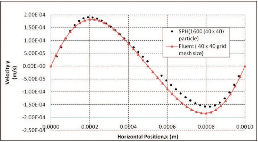
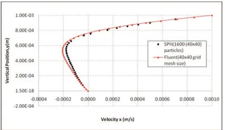
FIGURE 5. Distribution of 1600 (40 x 40) real particle after SPH simulation with a Reynolds Number of Re=1. Figure 6 and Figure 7 shows the dimensional vertical velocity profile along the horizontal centerline and the dimensional horizontal velocity profile along the vertical centerline respectively. The Fluent software results were obtained using a 40 x 40 grid mesh, which is comparable to the SPH resolution of 40 x 40 real particles. It can be seen from Figure 6 and Figure 7 that the results obtained using SPH is very close to the software Fluent results.
FIGURE 7. Horizontal velocity along the vertical centerline of the square cavity (x=0.005m) obtained using SPH method (present study) and software Fluent with a Reynolds Number of Re= 1.
However, the result might have the stability and accuracy problem. The solution is expected to converge closer than expected result by choosing another kernel function, addition of more particle use, using a different particle approximation, considering artificial viscosity, artificial heat and smoothing length evaluation[7-8].
CONCLUSION
The SPH method is used to discretize the Navier–Stokes equation that governs fluid flows. The methods have been examined and validated against a two-dimensional lid driven cavity problem. Results have shown that the problem using SPH method matched with the solution done by using software Fluent with both method are keeping the same properties to ensure they have same Reynolds numbers. It can be concluded that SPH is an attractive method for simulating incompressible flows with moving particles.
ACKNOWLEDGMENTS
We would like to thanks Universiti Teknologi Malaysia for providing facilities and Universiti Teknikal Malaysia for sponsoring this study.
REFERENCES
1. G. R. Liu, M. B. Liu, Smooth Particle Hydrodynamics - A Meshfree Particle Method, World Scientific Publishing Co. Pte. Ltd., 2007.
2. J. J. Monaghan, Annu. Rev. Astron. Astrophys. 30, 543–574 (1992).
3. M. Muller, D. Charypar and M. Gross, “Particle-based fluid simulation for interactive applications”, Proceedings of the 2003 ACM SIGGRAPH/Eurographics symposium on Computer animation, Aire-la-Ville, Switzerland, Eurographics Association, 2003, pp.154 159.
4. J. J. Monaghan, “Application of Smoothed Particle Hydrodynamics to Engineering Fluid Dynamics “,XVIII International Conference on Water Resources, 2010.
5. J. P. Morris, P. J. Fox, and Y. Zhu, Journal of Computational Physics136,214-226 (1997).
7. S. A. Osman and C. S. Nor Azwadi
, “UTOPIA Finite Difference Lattice Boltzmann Method for Simulation Natural Convection Heat Transfer from a Heated Concentric Annulus Cylinder”, European Journal of Scientific Research, 38, 2009, 63-71.