Mathematical Modelling Of Neill Mapping Function For Global Posittion System (GPS) Tropospheric Delay.

(1)

i

MATHEMATICAL MODELLING OF NEILL MAPPING FUNCTION FOR GLOBAL POSITION SYSTEM (GPS) TROPOSPHERIC DELAY

NOR AFIFAH BINTI ZAKARIA

This Report Is Submitted In Partial Fulfillment of Requirements for Degree of Bachelor in Electrical Engineering ( Mechatronics )

Faculty of Electrical Engineering

UNIVERSITI TEKNIKAL MALAYSIA MELAKA

(2)

ii

SUPERVISOR DECLARATION

“I hereby declared that I have read through this report and found that it has comply the partial fulfillment for awarding the Degree of Bachelor of Mechatronics Engineering

with Honours”

Signature : ____________________

Supervisor’s Name : Dr. Hamzah Bin Sakidin

(3)

iii

STUDENT DECLARATION

“I declare that this report entitle “Mathematical Modelling of Neill Mapping Function for Global Position System (GPS) Troposperic Delay” is the result of my own research except as cited in the references. The report has not been accepted for any degree and is not concurrently submitted in candidature of any other degree.

Signature : _____________________

Name : Nor Afifah Binti Zakaria

(4)

iv

DEDICATION

Dedicated to my beloved father and mother, my siblings, lecturers and to all my friends thanks

(5)

v

ACKNOWLEDGEMENT

Alhamdulillah thank to ALLAH S.W.T for his blessed at last I finished this Final Year Project. First of all, I would like to take this opportunity to express my gratitude to my supervisor; Dr. Hamzah Bin Sakidin for encouragement, support, critics and helps. Without his guidance and interest, this project wills not a success.

My sincere appreciation also extends to all my fellow friends for their assistance and motivation at the various occasions. Their views and tips are very useful indeed. Last but not least, thank you to all people who in one way or another contribute to the success of this project.

I am also grateful to all my family members.

(6)

vi

ABSTRACT

(7)

vii

ABSTRAK

(8)

viii

TABLE OF CONTENTS

SUPERVISOR DECLARATION ... ii

STUDENT DECLARATION ... iii

DEDICATION ... iv

ACKNOWLEDGEMENT ... v

ABSTRACT ... vi

ABSTRAK ... vii

TABLE OF CONTENTS ... viii

LIST OF FIGURES ... x

LIST OF TABLE ... xi

CHAPTER 1 ... 1

INTRODUCTION ... 1

1.1 Project Background ... 1

1.2 Problem Statement ... 2

1.3 Objective ... 3

1.4 Scope of project ... 3

1.5 Thesis outline ... 3

CHAPTER 2 ... 5

LITERATURE REVIEW ... 5

2.1 Introduction ... 5

2.2 Tropospheric Delay ... 5

2.3 Neill Mapping Function Model ... 6

2.4 Modification and simplification ... 9

(9)

ix

CHAPTER 3 ... 15

METHODOLOGY ... 15

3.1 Overview ... 15

CHAPTER 4 ... 26

RESULT ... 26

4.1 Introduction ... 26

4.2 Result For Hydrostatic Component ... 26

4.3 Result For Wet Component ... 29

4.5 Analysis For Wet Component ... 36

4.6 Discussion ... 39

CHAPTER 5 ... 41

CONCLUSION AND RECOMMENDATION ... 41

5.1 Conclusion ... 41

5.2 Recommendation For The Future Works ... 42

REFERENCES ... 43

APPENDICES ... 44

Appendix 1: Project Timeline (Fyp 1) ... 44

Appendix 2: Project Timeline (Fyp 2) ... 45

(10)

x

LIST OF FIGURES

Figure 2.1: Graph of NMFh mapping function (Y), Y1, Y2 and Y3 by regression ... 11

Figure 2.2: Graph of NMFw mapping function (Z), Z1, Z2 and Z3 by regression ... 13

Figure 3.1: Simulation process flow of the project flow ... 16

Figure 3.2: Step 1 ... 18

Figure 3.5: Comparison between modified and original model ... 21

Figure 3.6: Basic exponential graph. ... 22

Figure 3.7: Basic exponential function with B and C constant. ... 22

Figure 3.8: Exponential function with 3 constant A, B and C ... 23

Figure 3.9: Try and error method ... 23

Figure 3.10: Comparison graph between original and modification model ... 24

Figure 3.11: Table value of original and modified model ... 25

Figure 3.12: Table reduction percentage of the model operation ... 25

Figure 4.1: Modified model, N1 ... 28

Figure 4.4: Modified model, M1 ... 31

Figure 4.7: Graph comparison between modified and original hydrostatic model ... 34

Figure 4.8: Graph comparison deviation error for hydrostatic component ... 35

Figure 4.9: Graph comparison between modified and original wet model ... 37

(11)

xi

LIST OF TABLE

Table 2.1: Coefficients of the hydrostatic NMF mapping function [3] ... 7

Table 2.2: Coefficients of the wet NMF mapping function [3] ... 8

Table 2.3: Sum of error for NMFh, Y and simplified models (Y1, Y2, Y3) [2]... 10

Table 2.4: Sum of error for NMFw, Z and simplified models (Z1, Z2, Z3) [2] ... 12

Table 2.5: Reduction percentage of model operation ... 14

Table 4.1: Value of original and modified NMF models for hydrostatic component ... 27

Table 4.2: Value of original and modified NMF models for wet component ... 30

Table 4.3: Sum of error for NMF, N and modified models (N1, N2, N3) ... 33

Table 4.4: Sum of error for NMFw, M and modified models (MI, M2, M3) ... 36

(12)

1

CHAPTER 1

INTRODUCTION

1.1 Project Background

(13)

2

1.2 Problem Statement

The original mapping function model formula is more complex. As we know, the developed tropospheric delay models use mapping functions in the form of continued fractions which is quite tedious in calculation. There are 26 mathematical operations for Neill Mapping Function (NMF) which are very long to be calculated and difficult to understand. More time is needed to calculate the mapping function models to get the result. Neill Mapping Function, NMF as given in equation below [3]:

For hidrostatic component:

and for wet component:

Where:

- Elevation angle (degree)

NMFh()– Hydrostatic mapping function

NMFw()–Wet mapping function

(14)

3

1.3 Objective

There are three main objectives in this project which are:

i. To modify original model of the Neill mapping function. ii. To calculate the modified mapping function model.

iii. To compare the original NMF with the modified NMF result in term of the number of operation of the models.

1.4 Scope of project

In many study, there are some limits and constrain of the project that makes the project achievable. This project will be focused on the Neill mapping function models for both hydrostatics and non hydrostatics components. The software used to solve the problem is Maple 13 or excel software and lastly the elevation angle used between 3 to 90 only.

1.5 Thesis outline

This thesis consists of five chapters. It begins with introductory chapter. This chapter will discuss about background, problem statement, objective and scope of this project.

(15)

4 Chapter three will explain about methodology of this project. It is consisting software to find the modified NMF model by using maple13 and excel.

Chapter four will present the result as a project finding. In this chapter also, it will discuss about the analysis and discussion of the project. In the discussion part, it will explain how the original NMF models to be modified.

(16)

5

CHAPTER 2

LITERATURE REVIEW

2.1 Introduction

The purpose of a literature review is to convey the knowledge and ideas that have been established on this topic and also finding the strengths and weaknesses. Literature review has been conducted prior to undertaking this project to obtain the information on the technology available and technologies that used by the other researchers on the same topic around the world. This chapter provides the summary of literature reviews on key topics related Neill mapping function model.

2.2 Tropospheric Delay

The sum of several sources of error, such as orbit error, satellite clock error, multipath error, receiver noise error, selective availability, ephemeris error and also atmospheric error will determine the accuracy of Global Positioning System (GPS) measurement. Tropospheric delay is delay experienced by the GPS signal in propagating through the electrically neutral atmosphere. Usually, this delay will be calculated in the zenith direction and is referred to as a zenith tropospheric delay.

(17)

6

The mapping function depends on the elevation angles. The value of mapping function scale

factor equal to 1 (unity) is at 90 degree of elevation angle. So, this value will give minimum value for the tropospheric delay (TD) as given below [7]:

where:

ZHD is zenith hydrostatic delay (m) ZWD is zenith wet delay (m)

mh() is the hydrostatic mapping function ( - )

mw() is the wet mapping function ( - )

2.3 Neill Mapping Function Model

In this research, Neill Mapping Function model (NMF) are selected to be modified in order to reduce the computing time by reducing the percentage of number of operations.

In 1996, Arthur Neill already derive the mapping functions, are the most widely used, and are known to be the most accurate and easily-implemented functions. The new mapping function (NMF) is based on temporal changes and geographic location rather than on surface meteorological parameters. All previously available mapping functions have been limited in their accuracy by the dependence on surface temperature, which causes three dilemmas. There is more variability in temperature in the atmospheric boundary layer, from the Earth's surface up to 2000 m are the reason all these.

(18)

7 artificially large seasonal variations). Then, the computed mapping function for warm winter days may not significantly differ from function for cold summer days. For example, difference in lapse rates and heights of the troposphere will cause the actual mapping functions are quite different than computed values.

Temperature and relative humidity profiles, which are in some sense averages over broadly varying geographical regions can produce the new mapping functions. Niell compared NMF and ray traces calculated from radiosonde data spanning about one year or more covering a wide range of latitude and various heights above sea level [2]. The validity and applicability of the mapping function NMF can be identified by way of comparison.

We can see through the least-square fit of four different latitude data sets, Niell showed that the temporal variation of the hydrostatic mapping function is sinusoidal within the scatter of the data.

Table 2.1: Coefficients of the hydrostatic NMF mapping function [3]

Coefficients Latitude i

15° 30° 45° 60° 75°

Average

a 1.2769934e-3 1.2683230e-3 1.2465397e-3 1.2196049e-3 1.2045996e-3

b 2.9153695e-3 2.9152299e-3 2.9288445e-3 2.9022565e-3 2.9024912e-3

c 62.610505e-3 62.837393e-3 63.721774e-3 63.824265e-3 64.258455e-3

Amplitude

a 0.0 1.2709626e-5 2.6523662e-5 3.4000452e-5 4.1202191e-5

b 0.0 2.1414979e-5 3.0160779e-5 7.2562722e-5 11.723375e-5

c 0.0 9.0128400e-5 4.3497037e-5 84.795348e-5 170.37206e-5

Height correction

aht 2.53e-5

bht 5.49e-3

(19)

8

For the hydrostatic NMF mapping function, the parameter at tabular latitude i at time t

from January 0.0 (in UT days) is given below [3] :

where T0 is the adopted phase, DOY (day of year) 28. We can obtain the value of by

using the linear interpolation between the nearest . For parameters b and c, the same

procedure was followed.

Table 2.2: Coefficients of the wet NMF mapping function [3]

Coefficients

Latitude i

15° 30° 45° 60° 75°

aw 5.8021897e-4 5.6794847e-4 5.8118019e-4 5.9727542e-4 6.1641693e-4

bw 1.4275268e-3 1.5138625e-3 1.4572752e-3 1.5007428e-3 1.7599082e-3

cw 4.3472961e-2 1.5138625e-3 4.3908931e-2 4.4626982e-2 5.4736038e-2

The wet NMF mapping function not dependence to temporal. Therefore, requirement needed for each parameter is interpolation in latitude. Height correction associated with the NMF is given below [3]:

where is a three-term continued fraction and the parameters as

(20)

9

Before this, the large number of mapping functions was analyzed use data from 50 stations distributed worldwide (32,467 benchmark values). The models that meet the high standards of

modern space geodetic data analysis are Ifadis, Lanyi, MTT, and NMF. The models Lanyi, MTT, and NMF yield identical mean biases and the best total error performance at the elevation angle above 15 degrees Ifadis and NMF are superior at lower elevation angles.

The delay in the direction of an observation is related to the zenith delay by a mapping function to developed expression for calculating the ratios, which is modeled with sufficient

accuracy for elevations down to 3° using a three term continued fraction in sin  elevation,,

given by Neill Mapping Function, NMF as equation (1) for hydrostatic component and equation (2) for wet component.

2.4 Modification and simplification

The modification and simplication of NMF have been carried out as given below [2]:

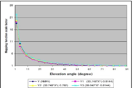
2.4.1 Hydrostatics Neill Mapping Function, NMFh ()

The same shape of graph for the original NMF is found by using regression method. The

original NMF () models is named as Y, while Y1, Y2, and Y3 are name for simplified

models. All four mapping function models give a graph of hyperbolic shape. However, there is a slightly difference between the Y model and the simplified models. The simplified model is such as below [2]:

(7)

where

Y1 : simplified NMFh()

A, B : constant

(21)

10

2.4.1.1 Sum of Error Calculation For NMFh ()

Table 2.3: Sum of error for NMFh, Y and simplified models (Y1, Y2, Y3) [2]

X Y = NMF(h) Y1 = 33.748* X(-0.8144) Y2 = 33.748* X(-0.782) Y3 = 39.042*

X(-0.8144) (Y -Y1)2 (Y -Y2)2 (Y -Y3)2

2 18.581 19.191 19.626 22.201 0.372 1.093 13.104

5 10.151 9.099 9.586 10.527 1.106 0.319 0.141

10 5.556 5.174 5.575 5.986 0.145 0.000 0.185

15 3.802 3.719 4.060 4.303 0.007 0.067 0.251

20 2.898 2.942 3.242 3.404 0.002 0.119 0.256

25 2.353 2.453 2.723 2.838 0.010 0.137 0.235

30 1.993 2.115 2.361 2.447 0.015 0.136 0.206

35 1.739 1.865 2.093 2.158 0.016 0.125 0.175

40 1.553 1.673 1.886 1.936 0.014 0.111 0.146

45 1.413 1.520 1.720 1.759 0.012 0.094 0.120

50 1.304 1.395 1.584 1.614 0.008 0.078 0.096

55 1.220 1.291 1.470 1.493 0.005 0.062 0.075

60 1.154 1.203 1.373 1.391 0.002 0.048 0.056

65 1.103 1.127 1.290 1.303 0.001 0.035 0.040

70 1.064 1.061 1.217 1.227 0.000 0.023 0.027

75 1.035 1.003 1.153 1.160 0.001 0.014 0.016

80 1.015 0.951 1.097 1.101 0.004 0.007 0.007

85 1.004 0.906 1.046 1.048 0.010 0.002 0.002

90 1.000 0.864 1.000 1.000 0.018 0.000 0.000

Sum of error 1.748 2.469 15.138

(22)

11

Figure 2.1: Graph of NMFh mapping function (Y), Y1, Y2 and Y3 by regression

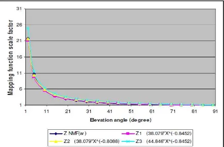
2.4.2 Wet Neill Mapping Function, NMFw()

Z is the NMFw () mapping function model, while the simplified model named as Z1, Z2, Z3.

There is a slight difference between the Z model and the three simplified model. These four models give the same shape of hyperbolic graph. The new model has been generated using regression method. We can reduce the computation time by using the simplification model. The simplified model is such as below [2]:

(8)

where

Z1: simplified NMFw().

A, B: constant

(23)

12

2.4.2.1 Calculation of Sum of Error For NMFw ().

Table 2.4: Sum of error for NMFw, Z and simplified models (Z1, Z2, Z3) [2]

X Z Z1= 38.079* X(-0.8452) Z2 = 38.079* X(-0.8088) Z3 = 44.846*

X(-0.8452) (Z - Z1)2 (Z - Z2)2 (Z - Z3)2

2 21.854 21.196 21.738 24.963 0.433 0.014 9.663

5 10.751 9.770 10.360 11.507 0.961 0.153 0.571

10 5.657 5.439 5.914 6.405 0.048 0.066 0.559

15 3.833 3.861 4.261 4.547 0.001 0.182 0.509

20 2.911 3.027 3.376 3.565 0.013 0.216 0.428

25 2.360 2.507 2.819 2.952 0.022 0.210 0.351

30 1.997 2.149 2.432 2.531 0.023 0.190 0.285

35 1.741 1.886 2.147 2.222 0.021 0.165 0.231

40 1.554 1.685 1.927 1.985 0.017 0.139 0.185

45 1.413 1.525 1.752 1.797 0.013 0.115 0.147

50 1.305 1.395 1.609 1.643 0.008 0.092 0.115

55 1.220 1.287 1.490 1.516 0.004 0.072 0.087

60 1.154 1.196 1.388 1.409 0.002 0.055 0.065

65 1.103 1.118 1.301 1.317 0.000 0.039 0.046

70 1.064 1.050 1.226 1.237 0.000 0.026 0.030

75 1.035 0.991 1.159 1.167 0.002 0.015 0.017

80 1.015 0.938 1.100 1.105 0.006 0.007 0.008

85 1.004 0.891 1.048 1.049 0.013 0.002 0.002

90 1.000 0.849 1.000 1.000 0.023 0.000 0.000

Sum of error 1.610 1.759 13.299

(24)

13

Figure 2.2: Graph of NMFw mapping function (Z), Z1, Z2 and Z3 by regression

2.5 Discussion and Conclusion