Volume 2010, Article ID 837360,18pages doi:10.1155/2010/837360
Research Article
Power Quality Analysis Using Bilinear
Time-Frequency Distributions
Abdul Rahim Abdullah
1and Ahmad Zuri Sha’ameri
21Faculty of Electrical Engineering, Technical university of Malaysia Malacca, 76100 Malacca, Malaysia 2Faculty of Electrical Engineering, Technical university of Malaysia, 81310 Johor, Malaysia
Correspondence should be addressed to Abdul Rahim Abdullah,[email protected]
Received 8 January 2010; Revised 4 June 2010; Accepted 8 December 2010
Academic Editor: Ulrich Heute
Copyright © 2010 A. R. Abdullah and A. Z. Sha’ameri. This is an open access article distributed under the Creative Commons Attribution License, which permits unrestricted use, distribution, and reproduction in any medium, provided the original work is properly cited.
Bilinear time-frequency distributions (TFDs) are powerful techniques that offer good time and frequency resolution of time-frequency representation (TFR). It is very appropriate to analyze power quality signals which consist of nonstationary and multi-frequency components. However, the TFDs suffer from interference because of cross-terms. Many TFDs have been implemented, and there is no fixed window or kernel that can remove the cross-terms for all types of signals. In this paper, the bilinear TFDs are implemented to analyze power quality signals such as smooth-windowed Wigner-Ville distribution (SWWVD), Choi-Williams distribution (CWD), B-distribution (BD), and modified B-distribution (MBD). The power quality signals focused are swell, sag, interruption, harmonic, interharmonic, and transient based on IEEE Std, 1159-1995. A set of performance measures is defined and used to compare the TFRs. It shows that SWWVD presents the best performance and is selected for power quality signal analysis. Thus, an adaptive optimal kernel SWWVD is designed to determine the separable kernel automatically from the input signal.
1. Introduction
Power quality is an issue that is becoming increasingly
important to electricity consumers at all levels of usage [1].
Poor power quality can cause very serious problems like
reduction of lifetime of the load, the ineffective performance
of protection devices, and instabilities and interruptions in manufacturing operation. For example, voltage sags to 80% of the nominal voltage with durations of 40 ms or greater would shut down the control electronics of production line
of an industrial plant [2]. Thus, there is a need for heightened
awareness of power quality among electricity users that require ultrahigh availability of service and precision man-ufacturing systems. Accordingly, an automated monitoring system is required to provide adequate coverage of the entire system, understand the causes of these disturbances, resolve
existing problems, and predict future problems [1]. Prompt
and accurate diagnosis of problems will ensure quality of power line signal, reduce diagnostic time in the presence of power disturbance, and rectify failures.
In the current research trend, short-time Fourier
trans-form (STFT) [3] is a popular technique for power quality
signals analysis. The technique presents the signals jointly in time-frequency representation (TFR) which provides tempo-ral and specttempo-ral information. However, it has the limitation of a fixed window width that results is a compromise between time and frequency resolution. The greater temporal resolution required, the worse frequency resolution will be and vice versa. To overcome the limitation of the fixed resolution of STFT, wavelet transform (WT) was proposed
by various researchers [4]. WT offers high time resolution
for high frequency component and high frequency resolution for low frequency component. Consequently, the technique is suitable to detect the duration of high frequency signal such as transient. For low frequency signal, typically sag, swell, and interruption, it does not produce reliable results
[5]. In addition, WT also exhibits some disadvantages such
as its computation burden, sensitivity to noise level, and the dependency of its accuracy on the chosen basis wavelet
Bilinear time-frequency distributions (TFDs) [7] have been intensively used to characterize and analyze
non-stationary signals. The bilinear TFDs offer a good time
and frequency resolution and are successfully applied to various real-life problems such as radar, sonar, seismic data analysis, biomedical engineering, and automatic emission.
However, the TFDs suffer from the presence of
cross-terms interferences because of its bilinear structure. This inhibits interpretation of its TFR, especially when signal has multiple frequency components. Some members of the bilinear TFDs are Wigner-Ville distribution (WVD), windowed Wigner-Ville distribution (WWVD), smooth-windowed Wigner-Ville distribution (SWWVD), Choi-Williams distribution (CWD), B-distribution (BD), mod-ified B-distribution (MBD), and Born-Jordan distribution (BJD). An analysis of the autoterms presentation using the reduced interference distributions (RID) has been discussed
in [8]. A procedure for designing a kernel that will produce
the desired autoterm shape and an optimal kernel with respect to the autoterm quality and cross-term were demon-strated.
In this paper, bilinear TFDs are implemented to analyze power quality signals. The popular bilinear TFDs are chosen such as SWWVD, CWD, BD, and MBD. To verify the performance of the TFDs, a set of performance measures is defined to compare the TFRs in terms of main-lobe width (MLW), peak-to-side lobe ratio (PSLR), absolute percentage error (APE), and signal-to-cross-terms ratio (SCR). From the comparison, the best bilinear TFD is chosen, and its adaptive optimal kernel system is designed. The adaptive system is to determine the optimal kernel parameters, automatically from the input signal, without prior knowledge of the signal. The optimal kernel is capable of removing the cross-terms, preserving the autoterms, and maintaining accurate TFR.
2. Power Quality Signal
According to the IEEE Standards 1159, electromagnetic phenomena are classified into several groups as shown in Table 1[9]. This paper focuses on six types of power quality signals: swell, sag, interruption, harmonic, interharmonic, and transient.
3. Signal Model
This paper divides the power quality signals into three classes. They are voltage variation for swell, sag, and in-terruption signal, waveform distortion for harmonic and interharmonic signal, and transient for transient signal. The signal models of the classes are formed as a complex expo-nential signal, and defined as
zvv(t)=ej2π f1t 3
k=1
AkΠk(t−tk−1), (1)
zwd(t)=ej2π f1t+Aej2π f2t, (2)
ztrans(t)=ej2π f1t 3
k=1
Πk(t−tk−1)
+Ae−1.25(t−t1)/(t2−t1)ej2π f2(t−t1)Π2(t
−t1), (3)
Πk(t)=
⎧ ⎨
⎩
1, for 0≤t≤tk−tk−1,
0, elsewhere, (4)
where zvv(t), zwd(t), and ztrans(t) are the voltage variation,
waveform distortion, and transient signal, respectively. kis
the signal component sequence,Akis the signal component
amplitude, f1and f2are the signal frequency,tis the time,
and Π(t) is a box function of the signal. In this analysis,
f1, t0, andt3 are set at 50 Hz, 0 ms, and 200 ms, and other
parameters are defined as follows:
(1) swell: A1 = A3 = 1,A2 = 1.2,t1 = 100 ms,t2 =
140 ms,
(2) sag:A1=A3=1,A2=0.8,t1=100 ms,t2=140 ms,
(3) interruption:A1 = A3 = 1,A2 = 0,t1 = 100 ms,
t2=140 ms,
(4) harmonic:A = 0.25, f2=250 Hz,
(5) interharmonic:A=0.25,f2=275 Hz,
(6) transient:A=0.5, f2 =1000 Hz,t1 =100 ms,t2 =
115 ms.
4. Bilinear Time-Frequency Distribution
Bilinear TFDs are powerful tools in the analysis of non-stationary and multicomponent signals. Many of these TFDs are invariant to time and frequency translations and can be considered as energy distribution in time-frequency domain
[10]. From the TFR, characteristics of the signals can be
calculated and used as input for signals classification. The signal characteristics are duration of swell, sag, interruption, and transient and average of total waveform distortion, total harmonic distortion, and total nonharmonic distortion. Further discussion of the signal characteristics can be found
in [11].
In general, the bilinear TFDs can be formulated as
Pzt,f= ∞
−∞G
(t,τ)∗
(t)Kz(t,τ) exp
−j2π f τ
dτ, (5)
whereG(t,τ) is the time-lag kernel function,Kz(t,τ) is the
bilinear product, and the asterisk witht denotes the time
convolution of the signals. The bilinear product is further defined as
Kz(t,τ)=z t+τ 2
z∗ t−τ
2
, (6)
where z(t) is the analytic signal of interest.
Smooth-windowed Wigner-Ville distribution (SWWVD) has a
sep-arable kernel [12] which is capable of reducing the effects of
Table1: Categories and typical characteristics of power system electromagnetic phenomena [9].
Categories Typical spectral content Typical duration Typical voltage magnitude 1.0 Transients
1.1 Impulsive
1.1.1 Nanosecond 5 ns rise <50 ns
1.1.2 Microsecond 1µs rise 50 ns–1 ms
1.1.3 Millisecond 0.1 ms rise >1 ms
1.2 Oscillatory
1.2.1 Low frequency <5 kHz 0.3–50 ms 0–4 pu
1.2.2 Medium frequency 5–500 kHz 20 ms 0–8 pu
1.2.3 High frequency 0.5–5 MHz 5 ms 0–4 pu
2.0 Short duration variations 2.1 Instantaneous
2.1.1 Sag 0.5–30 cycles 0.1–0.9 pu
2.1.2 Swell 0.5–30 cycles 1.1–1.8 pu
2.2 Momentary
2.2.1 Interruption 0.5 cycles–3s <0.1 pu
2.2.2 Sag 30 cycles–3s 0.1–0.9 pu
2.2.3 Swell 30 cycles–3s 1.1–1.4 pu
2.3 Temporary
2.3.1 Interruption 3 s–1 min <0.1 pu
2.3.2 Sag 3 s–1 min 0.1–0.9 pu
2.3.3 Swell 3 s–1 min 1.1-1.2 pu
3.0 Long duration variations
3.1 Interruption, sustained >1 min 0.0 pu
3.2 Undervoltages >1 min 0.8-0.9 pu
3.3 Overvoltages >1 min 1.1-1.2 pu
4.0 Voltage imbalance steady state 0.5–2%
5.0 Waveform distortion
5.1 DC offset Steady state 0–0.1%
5.2 Harmonics 0–100th H Steady state 0–20%
5.3 Interharmonics 0–6 kHz Steady state 0–2%
5.4 Notching Steady state
5.5 Noise Broad band Steady state 0–1%
6.0 Voltage fluctuations <25 Hz Intermittent 0.1–7%
7.0 Power frequency variations <10 s
a high time-frequency resolution. The general expression of the separable kernel is written as
G(t,τ)=H(t)w(τ), (7)
where H(t) is the time smooth (TS) function, w(τ) is the
lag window function, and its corresponding TFD can be expressed as
ρz,swwvdt,f= ∞
−∞H
(t)∗
(t)Kz(t,τ)w(τ)e
−j2π f τdτ. (8)
In this paper, Hamming window is used as the lag win-dow and raised-cosine pulse as the TS function. The
ham-ming window and the raised-cosine pulse [12] are defined as
w(τ)= ⎧ ⎪ ⎪ ⎨
⎪ ⎪ ⎩
0.54 + 0.46 cos
πτ Tg
, for−Tg ≤τ≤Tg,
0, elsewhere,
(9)
H(t)=
⎧ ⎪ ⎨
⎪ ⎩
1 + cos πt
Tsm
, for 0≤t≤Tsm,
0, elsewhere.
The lag window,w(τ), has a cutofflag atτ=Tg. The Doppler
representation of the TS function,H(t), that is obtained from
the Fourier transform with respect to time is
h(v)=sin(πvTsm)
πvTsm
+1
2
sin(π(v−1/2Tsm))
π(v−1/2Tsm)
+1
2
sin(π(v+ 1/2Tsm))
π(v+ 1/2Tsm) ,
(11)
where it is a low-pass filter in the Doppler domain, and the
cutoffDoppler frequency is
υc= 3
2Tsm
. (12)
The Choi-Williams distribution (CWD) kernel is
devel-oped to reduce interference in TFDs [7] and can be defined
as
G(t,τ)=
√πσ
|τ| e
−π2σt2/τ2
, (13)
whereσ is a real parameter that can control the resolution
and the cross-terms reduction [10]. This kernel has shown
good performance in reducing cross-terms while keeping high resolution with a compromise between these two requirements.
The B-distribution (BD) kernel [10] is defined in the
time-lag plane and can be expressed as
G(t,τ)= |τ|βcosh−2βt, (14)
whereβis a positive real parameter that controls the degree
of smoothing, and its value is between zero and unity. This kernel is a low-pass filter in the Doppler domain but not in the lag domain.
To improve the time resolution, the B-distribution was modified by making the lag-dependent factor exactly
constant [10]. The resulting modified B-distribution (MBD)
had a lag-independent kernel and can be defined as
G(t,τ)= cosh
−2βt ∞
−∞cosh−
2βξ dξ. (15)
5. Time-Lag Signal Characteristic
Generally, bilinear product of the signal interest is rep-resented in time-lag representation. The bilinear product consists of autoterms and cross-terms and can be defined as
Kz(t,τ)=Kz,auto(t,τ) +Kz,cross(t,τ). (16) In the time-lag representation, normally, the autoterms
are concentrated along the time axis and centered at τ =
0, while the cross-terms are located away from the axis. The autoterms must be preserved, while the cross-terms are suppressed by choosing appropriate kernel parameters. For SWWVD, TS function is used to remove Doppler frequency component existing in cross-terms, while lag window suppresses cross-terms that lie away from the origin
of the lag axis.Detail derivation of the autoterms and
cross-terms for all signals that are shown in (17) to (32) is derived
inAppendix A.
t1
t1
t2
t2
t3
t3
−t1
−t2
−t3
A1 A2 A3
A1,A2
A2,A1 A3,A2
A3,A1 −(t2−t1)
(t2−t1)
t
1
0 2 3
1, 2
A1,A3
A2,A3
1, 3
2, 3
2, 1
3, 1 3, 2
τ
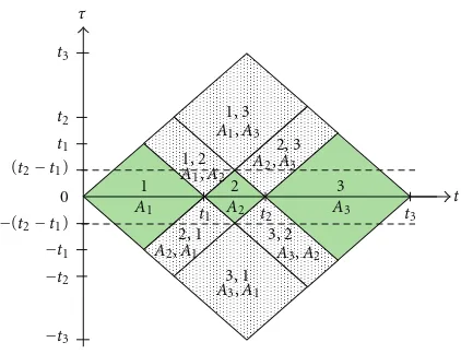
Figure 1: Bilinear product of the voltage variation signal. The autoterms are highlighted in green, while the cross-terms are densely dotted.
5.1. Bilinear Product of Voltage Variation Signal. Voltage
variation signal in (1) has a variation in the root mean square
(RMS) value from nominal voltage [9]. The autoterms and
cross-terms of this signal can be expressed as
Kauto,vv(t,τ)= 3
k=1
A2
kej2π f1τKΠk,k(t,τ),
Kcross,vv(t,τ)= 3
k=1 3
l=1 k /=l
AkAlej2π f1τKΠk,l(t,τ),
(17)
wherekandlrepresent the signal component sequence,Ak
andAlare the signal components amplitude, and the bilinear
product of the box function,Π(t), is defined as
KΠk,l(t,τ)=Πk t+
τ
2−tk
Πl t−τ
2−tl
. (18)
From (17), it is observed that the autoterms lie along the
time axis and are centered atτ =0, while the cross-terms are
elsewhere as shown inFigure 1.
For example, autoterm whenk=1 andl=1 is expressed
as
Kauto,vv t−t1
2,τ
=A2
1ej2π f1τKΠ1,1 t−
t1
2,τ
. (19)
This autoterm is located att = t1/2 and is centered at the
origin of the lag axis. It has a single lag-frequency component
which is at f = f1. Similar result is observed for autoterm
when k = 2 and l = 2. This autoterm which is at t =
t1/2 is also centered at the origin of the lag axis and has a
single lag-frequency component at f = f1. It can be defined
as
Kauto,vv t−t1+t2
2 ,τ
=A2
2ej2π f1τKΠ2,2 t−
t1+t2
2 ,τ
.
Meanwhile, for cross-term whenk = 1 andl = 2, it is
located att=(t2+ 2t1)/4 andτ=t2/2. The cross-term is due
to the interaction between 1st and 2nd signal component and
has only a single lag-frequency component at f = f1. It can
be expressed as
Kcross,vv t−t2
+ 2t1
4 ,τ−
t2 2
=A1A2ej2π f1τKΠ1,2 t−
t2+ 2t1
4 ,τ−
t2 2
.
(21)
Another example is cross-term which is due to the interaction between 2nd and 1st signal component. This
cross-term is centered att = (t2+ 2t1)/4 andτ =t2/2 and
also has only a single lag-frequency component at f = f1as
expressed in the following equation:
Kcross,vv t−t2
+ 2t1
4 ,τ+
t2 2
=A1A2ej2π f1τKΠ1,2 t−
t2+ 2t1
4 ,τ+
t2 2
.
(22)
The examples above prove that the autoterms are
cen-tered atτ = 0 and lie along the time axis, while the
cross-terms are elsewhere. Since the signal has only frequency
component at f = f1, it results that the autoterms and
cross-terms have a lag-frequency component at f = f1
and zero Doppler frequency. Thus, in order to suppress the cross-terms and to preserve the autoterms, lag window should cover all autoterms while removing the cross-terms
as much as possible. The lag window width,Tg, can be set
as
Tg
≤t2−t1. (23)
By using this limit, cross-terms such as whenk=1,l=2
andk=2,l=3 are preserved, since they are adjacent to the
autoterms as shown inFigure 1. The remaining cross-terms
can be reduced by using smallerTg, but it will compromise
the concentration of the autoterms. This results in smearing in frequency domain that reduces frequency resolution. In addition, the lag window width should contain at least one
cycle of fundamental signal such that Tg ≥ 1/2f1. The
actual effect of this setting will be discussed in the next
section.
Since the cross-terms do not have Doppler frequency, the use of the TS function will not contribute to the cross-terms suppression. Thus, the resulting TFD that uses a lag window and an impulse function as TS function is also known as windowed Wigner-Ville distribution (WWVD). It can be expressed as
ρz,wwvdt,f= ∞
−∞Kz(t,τ)w(τ)e
−j2π f τdτ, (24)
wherew(τ) is the lag window.
5.2. Bilinear Product of Waveform Distortion Signal. Wave-form distortion signal is a steady-state signal which consists
of multiple frequency components [13]. The autoterm and
cross-term of the signal in (2) can be defined as
Kauto,zwd(t,τ)=ej2π f1τ+A2ej2π f2τ, (25)
Kcross,zwd(t,τ)=2Aej2π((f2+f1)/2)τcos2πf2−f1t. (26)
As shown in (25), the autoterm is centered at the origin
of the lag axis and has two lag-frequency components which
are f1and f2. For the cross-term as shown in (26), it is also
centered at the origin of the lag axis. However, the cross-term
consists of a lag-frequency component at f =(f2+f1)/2 and
a Doppler frequency component atυ=(f2−f1).
Based on the observation, the Doppler frequency com-ponent only exists in the cross-term. TS function which is a low-pass filter in Doppler frequency domain can be used to remove the cross-term. Since the Doppler frequency
component is atυ=(f2−f1), the Doppler cutofffrequency
should be set atυc ≤ |f2− f1|. It can be achieved by setting
the TS function parameter,Tsm, as
Tsm≥ 3
2
f2−f1
. (27)
For signal that has more than two frequency components,
|f2−f1|is set as the smallest frequency deviation among the
signal frequency components. WhenTsmis set lower than the
limit in (27), the cutofffrequency will beυc>|f2− f1|that
will include the cross-term. Thus, the TS function will not be
able to remove the cross-term. Besides that, any higherTsm
value would result in a small cutoffDoppler frequency but
would cause the autoterm to smear in time. Thus,Tsmshould
be set at an appropriate value to remove the cross-term and avoid the smearing of autoterm in time.
Besides using the TS function to remove the cross-terms, lag window is also used to obtain desirable lag-frequency resolution in TFR. The lag-lag-frequency resolution
is set such that ∆f ≤ f1/2 to differentiate harmonic
and interharmonic frequency components. Therefore, the
lag window width should be set at Tg ≥ 1/2∆f. Higher
Tg offers higher lag-frequency resolution, but it increases
computation complexity and memory size to calculate TFR.
Thus,Tgshould be set at a sufficient value to obtain desirable
lag-frequency resolution and avoid higher computation complexity and memory size used. In this analysis, since
the signal fundamental frequency chosen is at f1 = 50 Hz,
Tg is set at minimum value which is 20 ms to reduce the
computation complexity and memory size of the analysis. It results in the fact that the lag-frequency resolution of the TFR
is∆f =25 Hz. In addition, the setting is also applicable for
all waveform distortion signals.
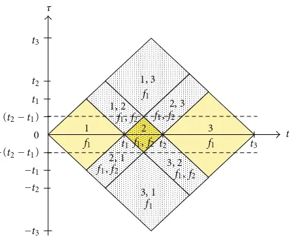
5.3. Bilinear Product of Transient Signal. Transient signal is a sudden signal which changes in steady-state condition at
nonfundamental frequency [9]. As indicated in transient
signal model in (3), there are three signal components. The
f1, while the second component has additional frequency
component which is transient frequency, f2. Thus, the
bilinear product of this signal produces three autoterms and seven cross-terms in time-lag representation as shown in Figure 2. The autoterms and cross-terms can be expressed as
Kauto,trans(t,τ)=ej2π f1τKΠ1,1(t,τ)
+ej2π f1τ+A2e−2.5(t−t1)ej2π f2τK
Π2,2(t,τ)
+ej2π f1τK
Π3,3(t,τ),
(28)
Ktrans,cross(t,τ)= 3
k=1 3
l=1 k /=l
ej2π f1τK
Πk,l(t,τ)
+ 3
l=1
Ae−1.25(t+τ/2−t1)ej2π(f2−f1)t−f2t1
×ej2π(f2+f1)τ/2K
Π2,l(t,τ)
+ 3
k=1
Ae−1.25(t+τ/2−t1)e−j2π(f2−f1)t−f2t1
×ej2π(f2+f1)τ/2K
Πk,2(t,τ).
(29)
Similar to the voltage variation signal, the autoterms in
(28) are centered atτ = 0 and lie along the time axis as
colored inFigure 2. For example, autoterm atk=1 is located
att=t1/2 and the origin of the lag axis. It has a lag frequency
at f = f1and can be defined as
Kauto,trans t−t1
2,τ
=ej2π f1τK
Π1,1 t−
t1
2,τ
. (30)
The location of the cross-terms in (29) is densely dotted
in Figure 2. The figure shows that cross-terms that are
generated by different signal components (k /=l) are located
away from the time axis, τ /=0. As example, a cross-term
defined in (31) is produced because of the interaction
between the first and second signal components (k=1 and
l = 2). It is centered att = (t2+ 2t1)/4 andτ = t2/2 and
has a Doppler frequency component atυ=(f2−f1) and two
lag-frequency components at f = f1and f =(f2+f1)/2:
Ktrans,cross t−t2
+ 2t1
4 ,τ−
t2 2
=ej2π f1τ+Ae−1.25(t+τ/2−t1)e−j2π(f2−f1)t−f2t1ej2π(f2+f1)τ/2
×KΠ1,2 t−
t2+ 2t1
4 ,τ−
t2 2
.
(31)
t1
t1
t2
t2
t3
t3
−t1
−t2
−t3 −(t2−t1)
(t2−t1)
t
1
0 2 3
1, 2 2, 3
2, 1
3, 1 3, 2
τ
f1
f1 f1
f1
f1,f2
f1,f2
f1,f2
f1,f2
f1,f2
1, 3
Figure2: Bilinear product of the transient signal.
The second signal component has two different
frequen-cies which are f1and f2. Its bilinear product can be defined
as
Kz2(t,τ)
=ej2π f1τ+A2e−2.5(t−t1)ej2π f2τ+ 2Ae−1.25(t+τ/2−t1)
×cos
j2π
f2−f1t−f2t1ej2π(f2+f1)τ/2
KΠ2,2(t,τ). (32)
This bilinear product introduces a cross-term which is
located att= (t2+t1)/2 and also centered atτ =0, where
it is similar to the autoterms. The cross-term has a Doppler
frequency component atυ = (f2− f1) and a lag frequency
component at f =(f2+ f1)/2 and can be defined as
Ktrans,cross t−t2
+t1
2 ,τ
=2Ae−1.25(t+τ/2−t1)ej2π(f2+f1)τ/2cosj2πf 2−f1
t−f2t1
×KΠ2,2 t−
t2+t1
2 ,τ
.
(33)
The purpose of using lag window in this signal is similar to the voltage variation signal. The lag window width is set
such that|Tg| ≤(t2−t1) to remove the cross-terms located
away from the time axis and to preserve the autoterms lying along the time axis. In addition, similar to the waveform distortion signal, TS function is also employed to remove the Doppler frequency component of the remaining cross-terms.
Since the Doppler frequency component isυ = (f2− f1),
the cutoffDoppler frequency of the TS function is set at
υc ≤ |f2− f1|by setting the TS function parameter, Tsm,
as in (27). An appropriate value of Tsm and Tg should be
Table2: Limit of the kernel parameters.
Signal Tg,min(ms) Tsm,min(ms)
Swell 10 0
Sag 10 0
Interruption 10 0
Harmonic 20 7.5
Interharmonic 20 6.67
Transient 10 1.578
5.4. Kernel Parameters. The analysis of bilinear product in time-lag representation to determine kernel parameters for all power quality signals is discussed in the previous subsections. Based on the analysis, the limits of the kernel
parameters as defined in (23) and (27) are summarized
in Table 2. The smallest lag window width, Tg,min, and TS
function parameter, Tsm,min, can be set in (9) and (10),
respectively, to obtain sufficient cross-terms suppression
with minimal autoterms bias as well as to reduce the computation complexity and memory size of the analysis.
6. Performance Comparison of
Kernel Parameters
Several performance measures are created and used to verify the TFR of the bilinear TFDs. They are main-lobe width (MLW), peak-to-side lobe ratio (PSLR), signal-to-cross-terms ratio (SCR), and absolute percentage error (APE). These measurements are adopted to evaluate concentration, accuracy, interference minimization, and resolution of TFRs
[12].
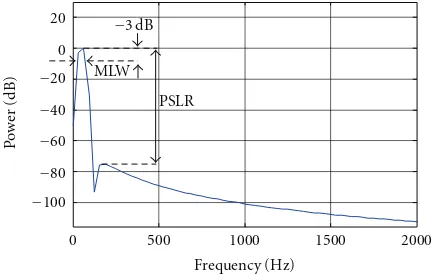
6.1. Performance Measurements. MLW and PSLR are calcu-lated from the power spectrum which is obtained from the
frequency marginal of the TFR [12] as shown in Figure 3.
MLW is the width at 3 dB below the peak of the power spectrum, while PSLR is the power ratio between the peak and the highest side lobe calculated in dB. Low MLW indicates good frequency resolution, and it gives the ability to resolve closely spaced sinusoids. PSLR should be as high as possible to resolve signal of various magnitudes.
SCR is a ratio of signal to cross-terms power in dB. High SCR indicates high cross-terms suppression in the TFR and is defined as
SCR=10 log
signal power
cross−terms power
. (34)
Besides the MLW, PSLR, and SCR, APE is also applied to quantify the accuracy of signal characteristics that are calculated from the TFR. This measurement has been
discussed in [11] and is expressed as
APE=xi−xm
xi ×
100%, (35)
where xi is actual value and xm is measured value. Low
APE shows high accuracy of the measurement. In general,
−100
−80 −60
−40
−20 0 20
Po
w
er
(d
B
)
0 500 1000 1500 2000
Frequency (Hz) PSLR
−3 dB
MLW
Figure3: Performance measures used in the analysis.
an optimal kernel of TFD should have low MLW and APE while high PSLR and SCR.
6.2. Performance Comparison of Smooth-Windowed Wigner-Ville Distribution. The performance of SWWVD with vari-ous kernel parameters for power quality signals is shown in Table 3. In this table, the kernel parameters are chosen based
on the observation made inSection 5. The bold values in
Table 3 presents the parameters that give optimal TFR for each type of signal. Even though, the discussion of the table will focus on transient signal and similar observation can be made for voltage variation and waveform distortion signal.
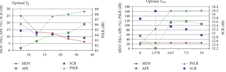
As shown in the table, the optimal kernel parameters for
the transient signal are atTg =10 ms andTsm =1.578 ms.
To observe the performance response corresponding to the kernel parameters, the performance measures of this signal
at optimalTsmwith variousTgand optimalTgwith various
Tsmare plotted inFigure 4.Figure 4(a)shows that, at optimal
Tsmand whenTgis set higher, the MLW is smaller indicating
a higher frequency resolution of the TFR. However, it suffers
from the reduction of the cross-terms suppression which
results in smaller SCR. This is because higherTgcovers more
adjacent cross-terms in lag axis in the bilinear product. As a result, the APE is higher which presents lower accuracy of the signal characteristic measurement. Since the fundamental
frequency, f1, is set at 50 Hz, the minimum Tg should be
set at 10 ms to cover at least one cycle of the fundamental signal.
At the optimal Tg and whenTsm is set higher than its
optimal value, the SCR increases, while the MLW remains
constant as shown inFigure 4(b). It indicates that higherTsm
improves the cross-terms suppression and does not give any
effect to the frequency resolution. However, the APE is also
higher which shows that the time resolution of the TFR is lower. This is because the application of TS function with
higherTsm increases the smearing of the autoterms in time
domain. Thus, there is a compromise between cross-terms suppression and time resolution to obtain optimal TFR.
The optimal kernel parameters for voltage variation
sig-nal are atTg =10 ms andTsm=0 ms. For this signal, the use
0 5 10 15 20 25 30
ML
W
(Hz),
AP
E
(%),
S
CR
(dB)
MLW APE
SCR PSLR
81 82 83 84 85 86 87 88 89
PSLR
(dB)
10 15 20 30 40 OptimalTg
(a) MLW, APE, PSLR, and SCR at optimalTsmwith variousTg
0 20 40 60 80 100 120 140 160 180
ML
W
(Hz),
AP
E
(%),
PSLR
(dB)
12.2 12.4 12.6 12.8 13 13.2 13.4 13.6 13.8 14 14.2 14.4
SCR
(dB)
0 1.578 6.67 7.5 10
MLW APE
PSLR SCR OptimalTsm
(b) MLW, APE, PSLR, and SCR at optimalTgwith variousTsm
Figure4: Performance of the TFR using SWWVD with various kernel parameters for transient signal. (The kernel parameters chosen must give low MLW and APE but high PSLR and SCR.)
Table3: Performance comparison of SWWVD with various kernel parameters.
Kernel Parameters Performancemeasures
Signal
Voltage variation signal Waveform distortion signal Transient signal Swell Sag Interruption Harmonic Interharmonic Transient
Tg=10 ms
Tsm=0 ms
MLW (Hz) 25 25 25 25 25 25
PSLR (dB) 614.82 614.82 614.82 623.12 50.795 19.102
SCR (dB) 15.641 17.799 55.446 4.4785 4.5758 13.764
APE (%) 0.2083 0.625 0.625 0.3755 100 55
Tg=40 ms
Tsm=0 ms
MLW (Hz) 6.25 6.25 6.25 6.25 6.25 6.25
PSLR (dB) 117.60 117.55 89.657 644.84 652.71 86.259
SCR (dB) 8.9462 11.216 48.903 9.0262 9.0721 9.4476
APE (%) 1.4583 1.875 1.0417 141.27 25.031 19.444
Tg=10 ms
Tsm=1.578 ms
MLW (Hz) 25 25 25 25 25 25
PSLR (dB) 218.09 216.68 198.78 18.835 49.889 86.145
SCR (dB) 13.491 15.038 35.107 5.6064 5.7679 14.171
APE (%) 3.125 12.708 100 55.544 100 1.6667
Tg=15 ms
Tsm=1.578 ms
MLW (Hz) 13.333 13.333 13.333 13.333 13.333 13.333
PSLR (dB) 130.99 130.68 127.89 17.623 17.712 84.025
SCR (dB) 11.751 13.297 33.514 10.959 11.289 12.567
APE (%) 69.791 117.08 100 100 100 6.6667
Tg=20 ms
Tsm=6.67 ms
MLW (Hz) 12.5 12.5 12.5 12.5 12.5 12.5
PSLR (dB) 229.98 228.53 210.04 51.168 638.24 154.53
SCR (dB) 9.8581 11.485 31.371 27.934 23.752 10.442
APE (%) 14.583 29.375 100 20.142 0.125 107.78
Tg=40 ms
Tsm=6.67 ms
MLW (Hz) 6.25 6.25 6.25 6.25 6.25 6.25
PSLR (dB) 120.03 100.92 81.315 51.168 655.78 129.74
SCR (dB) 6.7221 8.4121 28.701 28.570 24.256 7.7198
APE (%) 20.416 35.417 100 20.142 0.125 90.556
Tg=20 ms
Tsm=7.5 ms
MLW (Hz) 12.5 12.5 12.5 12.5 12.5 12.5
PSLR (dB) 229.97 228.53 209.88 643.28 68.843 156.11
SCR (dB) 9.8073 11.439 31.289 41.007 31.001 10.248
APE (%) 16.666 31.667 100 0.125 1.4268 115
Tg=40 ms
Tsm=7.5 ms
MLW (Hz) 6.25 6.25 6.25 6.25 6.25 6.25
PSLR (dB) 122.91 102.56 111.22 664.29 651.32 131.79
SCR (dB) 6.6568 8.3551 28.600 41.739 32.356 7.4996
Table4: Performance comparison of Choi-Williams distribution.
Signal
Kernel Parameters Performance
measures Voltage variation signal Waveform distortion signal Transient signal Swell Sag Interruption Harmonic Interharmonic Transient
σ=1.0
MLW (Hz) 2.34375 2.34375 2.34375 2.34375 2.34375 2.34375
PSLR (dB) 66.6589 66.6589 66.6589 45.5389 47.4593 67.5132
SCR (dB) 5.61185 7.81444 28.6804 21.4932 22.3112 7.0376
APE (%) 2.70833 3.54166 81.8750 59.5457 59.0395 21.6667
σ=0.5
MLW (Hz) 2.34375 2.34375 2.34375 2.34375 2.34375 2.34375
PSLR (dB) 78.8655 78.8655 78.8655 45.1447 47.3009 81.7881
SCR (dB) 5.51383 7.68141 27.6884 22.9633 23.9232 6.75077
APE (%) 1.45833 2.29166 85.2083 53.8937 55.8645 34.4444
σ=0.1
MLW (Hz) 2.34375 2.34375 2.34375 2.34375 2.34375 2.34375
PSLR (dB) 51.309 51.309 51.309 45.3051 52.875 51.9201
SCR (dB) 6.0203 8.1977 27.1346 25.3153 26.4656 6.22225
APE (%) 0.20833 0.62500 63.7500 49.3376 49.6516 49.4444
σ=0.05
MLW (Hz) 2.34375 2.34375 2.34375 2.34375 2.34375 2.34375
PSLR (dB) 52.0779 52.0779 52.0779 47.666 49.1118 53.6057
SCR (dB) 6.53223 8.73298 27.4525 26.7083 27.7299 6.30179
APE (%) 0.20833 0.20833 56.8750 44.1498 43.7457 52.2222
σ=0.01
MLW (Hz) 5.85938 5.85938 5.85938 4.6875 4.6875 4.6875
PSLR (dB) 57.8314 57.8314 57.8314 59.4144 61.5886 67.2973
SCR (dB) 8.18709 10.4501 28.9207 30.6248 31.5286 7.20599
APE (%) 0.62500 0.41666 75.0000 15.5563 28.2073 51.6667
σ=0.005
MLW (Hz) 5.85938 5.85938 5.85938 5.85938 5.85938 5.85938
PSLR (dB) 45.6061 45.6061 45.6061 62.4682 54.3076 57.5039
SCR (dB) 9.03793 11.3288 29.758 30.8003 32.5905 7.8471
APE (%) 1.04166 0.62500 78.3333 13.1708 24.7269 48.8889
σ=0.001
MLW (Hz) 9.375 9.375 9.375 9.375 9.375 9.375
PSLR (dB) 53.3157 53.3157 53.3157 60.5077 56.1806 58.7548
SCR (dB) 11.2395 13.5999 32.0283 29.0768 30.1635 9.93482
APE (%) 1.45833 1.25000 83.3333 2.36060 12.7563 49.4444
Doppler frequency. In addition, higherTsmreduces the time
resolution of the TFR. Therefore, as theTsmis set higher, the
SCR is lower, and APE is higher. For waveform distortion signal, the optimal kernel parameters for harmonic signal are
at Tg = 20 ms andTsm = 7.5 ms while for interharmonic
signal are at Tg = 20 ms and Tsm = 6.67 ms. All
cross-terms of these signals have Doppler frequency and can be
removed by using the TS function at the optimalTsm. Higher
Tg does not improve the cross-terms suppression. However,
it is still used to set the frequency resolution of the TFR
that can differentiate between harmonic and interharmonic
frequency components.
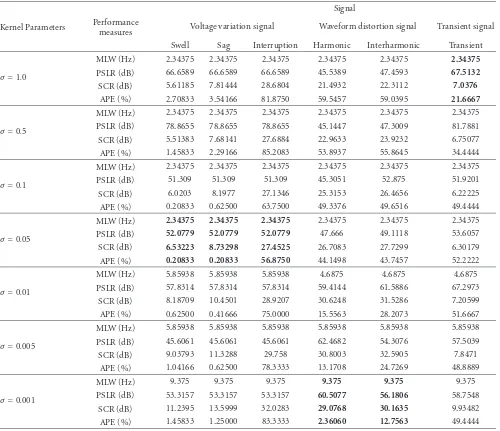
6.3. Performance Comparison of Choi-Williams Distribution.
Performance of the CWD is also compared with various
kernel parameters. The kernel parameter, σ, is set at 1.0,
0.05, 0.1, 0.05, 0.01, 0.005, and 0.001 as shown inTable 4.
This table shows that the optimal parameter for voltage
variation, waveform distortion, and transient signal is atσ =
0.05, 0.001, and 1.0, respectively.
All signals present similar performance response whenσ
is set higher or smaller than their optimal value. As example,
the performance measures of sagsignal using various σ is
shown graphically in Figure 5. The graph illustrates that,
whenσ is set higher than its optimal kernel, the MLW and
SCR are smaller. Higherσincreases frequency resolution of
the TFR, but it reduces cross-terms suppression. As a result,
the APE is higher. As σ is set smaller, the SCR is higher
because smallerσ removes more cross-terms. However, the
frequency and time resolution get worse, resulting in higher
MLW and APE. Thus,σshould be chosen based on the signal
0
Figure5: Performance comparison of the TFR using CWD with variousσfor sag signal.
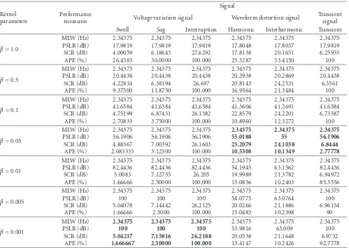
Table5: Performance comparison of B-distribution.
Signal Kernel
parameters
Performance
measures Voltage variation signal Waveform distortion signal
Transient signal Swell Sag Interruption Harmonic Interharmonic Transient
β=1.0
6.4. Performance Comparison of B-Distribution. BD is
another TFD used in this paper. Table 5 presents the
performance of the TFD with various kernel parameters,
β, at 1.0, 0.05, 0.1, 0.05, 0.01, 0.005, and 0.001. The result
shows that the optimal kernel for voltage variation signal is at
β=0.001 while waveform distortion and transient signal are
atβ=0.05. For all signals, asβis set other than the optimal
value, the MLW is similar, and the SCR is smaller. This
indicates thatβdoes not change the frequency resolution and
reduce the cross-terms suppression in the TFR. As a result, the APE is higher. The trends of this performance are shown inFigure 6which proves that the optimal kernel of harmonic
is atβ=0.05.
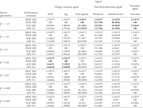
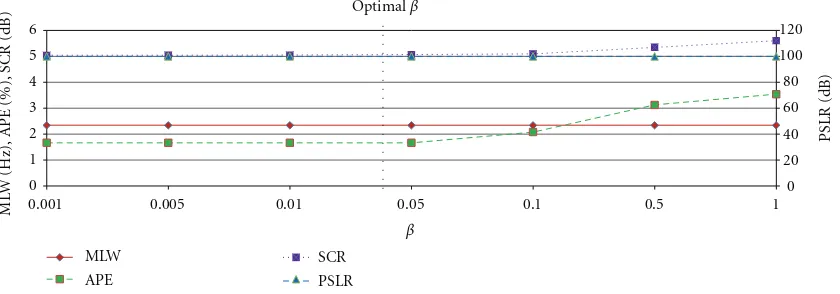
6.5. Performance Comparison of Modified B-Distribution.
PSLR
Figure6: Performance comparison of the TFR using BD with variousβfor harmonic signal.
Table6: Performance comparison of modified B-distribution.
Signal
Voltage variation signal Waveform distortion signal Transient signal Kernel
parameters
Performance
measures Swell Sag Interruption Harmonic Interharmonic Transient
β = 1.0
to BD as shown inTable 6. The table shows that the optimal
kernel parameter for swell and sag is β = 0.05 while for
interruption, harmonic, interharmonic, and transient signals
isβ=1.0. For instance,Figure 7shows the performance of
swell signal using variousβand its optimal value is identified
atβ=0.05.
7. Adaptive Optimal Kernel
In the previous section, the performance of SWWVD, CWD, BD, and MBD is analyzed with various kernel parameters. From the analysis, the optimal performance of the
PSLR
Figure7: Performance comparison of the TFR using MBD with variousβfor swell signal.
Table7: Performance comparison between optimal kernel parameters for the TFDs.
Signal SWWVD CWD BD MBD
Voltage
variation signal Swell
MLW (Hz)
Kernel parameter Tg=10 ms
Tsm=0 ms σ=0.05 β=0.001 β=0.05
Kernel parameter Tg=10 ms
Tsm=0 ms σ=0.05 β=0.001 β=0.05
Kernel parameter Tg=10 ms
Tsm=0 ms σ=0.05 β=0.001 β=1.0
Waveform
distortion signal Harmonic
MLW (Hz)
Kernel parameter Tg=10 ms
Tsm=1.58 ms
The result shows that the SWWVD is the best distribution for power quality signal analysis and an adaptive optimal kernel for SWWVD is designed.
Based on the analysis in Sections5and6, a guideline to
determine the separable kernel parameters of SWWVD for power quality signals is given as follows.
(i) For voltage variation signal
Tg =10 ms, Tsm=0 ms. (36)
(ii) For waveform distortion signal
Tg =20 ms, Tsm= 3
2
f2−f1
. (37)
(iii) For transient
Tg =10 ms, Tsm=
3
2
f2−f1
. (38)
The kernel parameters are different based on the
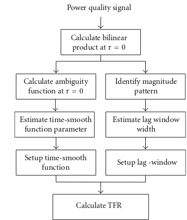
char-acteristics of the signals. Hence, an adaptive kernel system is required which is capable of setting the kernel parameters automatically from input signal. In this paper, based on the kernels setting given above, the adaptive kernel system for
power quality signal is designed as shown inFigure 8.
Firstly, bilinear product atτ = 0 for the input signal is
calculated. It can also be called instantaneous energy of the
interest signal,x(t) [14], and can be expressed as
Kx(t, 0)=x(t)x∗(t). (39)
For the signal models in (1) to (3), the bilinear product
atτ = 0 of the voltage variation, waveform distortion, and
transient signal are, respectively, defined as
Kz,vv(t, 0)= 3
k=1
A2
kΠk(t−tk),
Kz,wd(t, 0)=1 +A2+ 2Acos2πf2−f1t,
Kz,trans(t, 0)= 3
k=1
Πk(t−tk)
+A2e−2.5(t−t1)+ 2Ae−1.25(t+τ/2−t1)
×cos
j2π
f2−f1t−f2t1Π2(t−t2). (40)
The above equations show that the voltage variation and transient signal have a momentary energy variation between
t1andt2, while the waveform distortion has no momentary
energy variation. Thus, based on this observation and the
guideline given in (36) to (38), the lag window width is set
at Tg = 10 ms for the signal that has momentary energy
variation, while, for no momentary energy variation,Tg is
set at 20 ms.
In process to estimate TS function parameters, Tsm,
ambiguity function of the bilinear at τ = 0 is employed.
Power quality signal
Calculate bilinear product atτ=0
Calculate ambiguity function atτ=0
Estimate time-smooth function parameter
Setup time-smooth function
Calculate TFR
Identify magnitude pattern
Estimate lag window width
Setup lag -window
Figure8: Process flow of the adaptive optimal SWWVD.
It is calculated by using (41) to present the Doppler frequency
component of the bilinear product. From the ambiguity
function, the lowest Doppler frequency, υmin, is identified
and used to calculateTsmas defined in (42):
Az(υ, 0)= ∞
−∞Kz
(t, 0)e−j2πυtdt, (41)
Tsm=
3
2υmin
. (42)
As indicated in (40), the waveform distortion and
tran-sient signal have a Doppler frequency component atυ= |f2−
f1|while the voltage variation has zero Doppler frequency.
Thus, for waveform distortion and transient signal, υmin is
set at |f2− f1| and is then used in (42) to calculate Tsm.
Since the voltage variation has no Doppler frequency, the
time-smooth function parameter is set at Tsm = 0 ms, or,
in other words, the TS function used is a delta function. For normal signal, it has zero Doppler frequency as well as no energy variation. Therefore, the kernel parameters used are
similar to the voltage variation signal which areTg =10 ms
andTsm=0 ms. Finally, the setting of the kernels is used to
calculate the SWWVD to represent the signal in TFR.
For example, Figures9to11show swell, harmonic, and
transient signals and their bilinear product and ambiguity
function at τ = 0, respectively. As shown in Figure 9(a),
the magnitude of the swell signal is 1.2 pu starting from 100
to 140 ms, whileFigure 9(b)shows that its energy increases
from 1 to 1.44 pu between 100 and 140 ms. The signal
has zero Doppler-frequency as shown in Figure 9(c). For
harmonic signal inFigure 10(a), it is a constant sinusoidal
energy as shown in Figure 10(b), whileFigure 10(c) shows
its Doppler frequency isυ =200 Hz. It is different from the
transient signal that has a short energy variation between 100
and 115 ms, while its Doppler frequency is atυ=950 Hz as
−1 0 1
A
m
plitude
0 50 100 150 200
Signal
Time (ms)
(a)
0 50 100 150 200
0.5 1 1.5
Bilinear product atτ=0
Time (ms)
Energ
y
(b)
0 0.5 1
Energ
y
0 2000 4000 6000 8000 10000 12000
Doppler -frequency (Hz) Ambiguity function atτ=0
(c)
Figure9: (a) Swell signal, (b) its bilinear product, and (c) ambiguity function atτ=0.
Based on the adaptive system design, since the bilinear
product at τ = 0 of swell and transient signals has a
momentary energy variation, the lag window width is set at
Tg = 10 ms. For harmonic signal that has no momentary
energy variation, the lag window width is set at Tg =
20 ms. The harmonic and transient signals have a Doppler frequency. Thus, the values of the Doppler frequency are
used in (42) to calculateTsm. As a result, the setting ofTsm
for the harmonic and transient signals is 7.5 and 1.578 ms, respectively. For the swell signal, it has no Doppler frequency
component, andTsmis set at 0 ms.
8. Results
In this section, the results of the power quality analysis using SWWVD, CWD, BD, and MBD are discussed. The example of the signals and their TFRs using the TFDs at optimal
kernels is shown in Figures12to15. The line graphs show
the signal in time domain, while the contour plots show the TFR. The highest power is represented in red color while the lowest in blue color.
Figure 12shows a sag signal and its TFR using SWWVD. The magnitude of the sag signal is 0.8 pu, while its duration is between 100 and 140 ms. The contour plot presents that there is a momentary decrease of power at 50 Hz
(fundamental frequency) from 100 to 140 ms. InFigure 13,
there is a harmonic signal in time domain and its TFR
A
m
plitude
−2 0 2
0 20 40 60 80 100 120 140 160 180 200 Time (ms)
Signal
(a)
0 20 40 60 80 100 120 140 160 180 200 Time (ms)
0 0.5 1 1.5
Energ
y
Bilinear product atτ=0
(b)
Energ
y
0 0.02 0.04 0.06
0 50 100 150 200 250 300 350 400 450 500
Doppler -frequency Ambiguity function atτ=0
(c)
Figure10: (a) Harmonic signal, (b) its bilinear product, and (c) ambiguity function atτ=0.
by using CWD. The TFR shows that the harmonic signal consists of two frequency components which are 50 and 250 Hz.
A swell signal and its TFR using BD are shown in Figure 14. The magnitude of the swell signal is 1.2 pu between 100 and 140 ms. The TFR shows that the power increases from 120 to 160 ms, and its frequency is 50 Hz. The last example is transient signal. This signal and its TFR using
MBD are shown inFigure 15. The transient signal begins at
100 ms, and its duration is 15 ms. In the contour plot, the transient power increases between 118 and 125 ms, and its frequency is 1000 Hz.
In the contour plots, the TFRs show some delays com-pared to the input signals. This is because the convolution process between kernel and signal in the TFDs shifts the TFRs in time domain. For the TFR of sag signal using SWWVD, there is no delay because the kernel parameter used for
time-smooth function is set at Tsm = 0 ms. Generally,
this observation clearly shows that the TFRs represent the characteristics of the power quality signals.
By assuming perfect knowledge of the power quality signals, the performance of the bilinear TFDs with various
kernel parameters has been analyzed as shown in Tables3to
6. From those tables, the optimal performance of the TFDs is
identified and summarized inTable 7.
0 20 40 60 80 100 120 140 160 180 200
Bilinear product atτ=0
Energ
700 750 800 850 900 950 1000 1050 1100 1150 1200
Doppler -frequency Ambiguity function atτ=0
Energ
y
×10−4
(c)
Figure11: (a) Harmonic signal, (b) its bilinear product, and (c) ambiguity function atτ=0.
1
gives good APE, SCR, and PSLR while MLW is poor. For
CWD, BD, and MBD, they offer good MLW but poor APE,
Table8: Performance comparison between optimal and adaptive optimal kernel parameters.
Signal Performance
measures Optimal Adaptive
Voltage
For any unknown signal, an adaptive optimal kernel
SWWVD system is designed as discussed in Section 7 to
determine automatically the optimal kernel parameters. Then, the performance of the adaptive kernel is identified and compared with the performance of the optimal kernel
as shown inTable 8.
This table shows that, for every signal, the adaptive kernel gives similar parameters to the optimal kernel. As a result, the performance of adaptive kernel is comparable to the performance of optimal kernel. In addition, the adaptive system also gives high accuracy for the measurement of the
signal characteristics as discussed inSection 6.1. Therefore,
the adaptive kernel system is suitable to be implemented for power quality analysis as well as for classification pur-pose.
The performance of SWWVD for power quality signals
classification in noisy condition has been discussed in [15].
A set of 100 signals with various characteristics for each type of power quality signal were generated and classified
at SNR from 0 to 40 dB. The results show that the system can classify all signals without error at 36 dB of SNR and above.
9. Conclusions
This paper presents the analysis of power quality signals using SWWVD, CWD, BD, and MBD to identify the optimal kernel parameters. The performance measures used are
MLW, PSLR, SCR, and APE. The results show that different
power quality signals need different kernel parameters for
optimal TFR. There is no one kernel parameter that can be used optimally for all signals.
At the optimal kernel setting, the SWWVD gives the best performance of TFR compared to the other TFDs, and its adaptive optimal kernel is designed. The adaptive system can obtain optimal kernel setting automatically without prior knowledge of the signal. The result shows that the adaptive kernels system is comparable to the optimal kernel and is suitable for power quality analysis and classification purpose.
Appendices
The bilinear product that is given in (6) represents a signal
in time-lag representation. This representation consists of
two terms: autoterms and cross-terms as defined in (16).
This section discusses the calculation of bilinear product to obtain the autoterms and cross-terms for the power quality signals.
A. The Voltage Variation Signal
The voltage variation signal in (1) has three sequence signals
at fundamental frequency,f1, and its bilinear product is given
as
the time,kand lare the signal sequence starting with one,
and Π(t) is a box function of the signal as expressed in
The autoterms are bilinear product of a signal with the
same signal,k = l. Thus, the autoterms for this signal are
defined as
The cross-terms are bilinear product between different
signal,k /=l, and expressed as
B. The Waveform Distortion Signal
The waveform distortion signal in (2) is different from the
previous signal that has one signal and consists of two
frequency components, f1 and f2. Its bilinear product is
expressed as
The function above shows that the autoterms have two
lag-frequency components similar to the signal frequencies, f1
and f2frequencies, while the cross-terms exist in the middle
between the lag-frequency components, (f2+f1)/2, and have
a Doppler frequency atυ= f2−f1. The autoterms and
cross-terms are defined as
Kauto,zwd(t,τ)=ej2π f1τ+A2ej2π f2τ,
Kcross,zwd(t,τ)=2Aej2π((f2+f1)/2)τcos2πf2−f1t. (B.2)
C. The Transient Signal
The transient signal in (3) has three sequence signals. The
first and third signals are normal signal at fundamental
frequency,f1, while the second signal has additional transient
frequency,f2. The bilinear product of this signal is defined as
Kz,trans(t,τ)=
As discussed for the voltage variation and waveform distor-tion signal, autoterms and cross-terms of transient signal can be defined as
Acknowledgments
The authors would like to thank Technical university of Malaysia Malacca (UTeM) for its financial support and Technical university of Malaysia for providing the resources for this research.
References
[1] D. B. Vannoy, M. F. McGranaghan, S. M. Halpin, W. A. Mon-crief, and D. D. Sabin, “Roadmap for power-quality standards development,” IEEE Transactions on Industry Applications, vol. 43, no. 2, pp. 412–421, 2007.
[2] R. B. Godoy, J. O. P. Pinto, and L. Galotto Jr., “Multiple signal processing techniques based power quality disturbance detection, classification, and diagnostic software,” in Proceed-ings of the 9th International Conference on Electrical Power Quality and Utilisation (EPQU ’07), pp. 1–6, Barcelona, Spain, October 2007.
[3] K.-K. Poh and P. Marziliano, “Analysis of neonatal EEG signals using stockwell transform,” in Proceedings of the IEEE International Conference on Engineering in Medicine and Biology Society (EMBS ’07), pp. 594–597, Lyon, France, August 2007.
[4] Z. Shi, L. Ruirui, W. Qun, J. T. Heptol, and Y. Guimin, “The research of power quality analysis based on improved S-transform,” inProceedings of the 9th International Conference
on Electronic Measurement and Instruments (ICEMI ’09),
vol. 2, pp. 2477–2481, Beijing, China, August 2009.
[5] T. Radii, P. M. Ramos, and A. C. Serra, “Detection and extraction of harmonic and non-harmonic power quality disturbances using sine fitting methods,” in Proceedings of the 13th International Conference on Harmonics and Quality
of Power (ICHQP ’08), pp. 1–6, Wollongong, Australia,
September 2008.
[6] F. Zhao and R. Yang, “Power-quality disturbance recognition using S-transform,” IEEE Transactions on Power Delivery, vol. 22, no. 2, pp. 944–950, 2007.
[7] B. Barkat and B. Boashash, “A high-resolution quadratic time-frequency distribution for multicomponent signals analysis,”
IEEE Transactions on Signal Processing, vol. 49, no. 10, pp. 2232–2239, 2001.
[8] L. Stankovi´c, “Auto-term representation by the reduced inter-ference distributions: a procedure for kernel design,” IEEE Transactions on Signal Processing, vol. 44, no. 6, pp. 1557–1563, 1996.
[9] “IEEE recommended practice for monitoring electrical power quality,” IEEE Standards 1159-1995 Approved, June 1995. [10] B. Boashash,Time-Frequency Signal Analysis and Processing:
A Comprehensive Reference, Elsevier, Amsterdam, The Nether-lands, 2003.
[11] A. R. Abdullah and A. Z. Sha’ameri, “Power quality analy-sis using linear time-frequency distribution,” in Proceedings of the 2nd IEEE International Power and Energy Confer-ence (PECon ’08), pp. 313–317, Johor, Malaysia, December 2008.
[12] J. L. Tan and A. Z. B. Sha’Ameri, “Adaptive optimal kernel smooth-windowed wigner-ville distribution for digital com-munication signal,”EURASIP Journal on Advances in Signal Processing, vol. 2008, Article ID 408341, 2008.
[13] A. Moreno, Power Quality: Mitigation Technologies in a Distributed Environment, Springer, New York, NY, USA, 2007.
[14] Z. Sharif, M. S. Zainal, A. Z. Sha’ameri, and S. H. S. Salleh, “Analysis and classification of heart sounds and murmurs based on the instantaneous energy and frequency estima-tions,” inProceedings of the IEEE International Conference on Intelligent System and Technologies for the New Millennium (TENCON ’00), vol. 2, pp. 130–134, Kuala Lumpur, Malaysia, September 2000.
![Table 1: Categories and typical characteristics of power system electromagnetic phenomena [9].](https://thumb-ap.123doks.com/thumbv2/123dok/576990.68446/3.600.56.548.83.548/table-categories-typical-characteristics-power-electromagnetic-phenomena.webp)