SHRINKAGE ESTIMATION OF MEAN VARIANCE PO

(1)

Vol. 19, No. 1 (2016) 1650003 (25pages) c

World Scientific Publishing Company DOI:10.1142/S0219024916500035

SHRINKAGE ESTIMATION OF MEAN-VARIANCE PORTFOLIO

YAN LIU Department of Finance Ocean University of China No. 238 Song Ling Road, Qing Dao

Shan Dong 266100, P. R. China liuyan ouc@126.com

NGAI HANG CHAN∗

Department of Statistics The Chinese University of Hong Kong N.T. Shatin, Hong Kong, P. R. China

nhchan@sta.cuhk.edu.hk

CHI TIM NG Department of Statistics Chonnam National University

77 Yongbong-ro, Buk-gu Gwangju 500-757, Republic of Korea

easterlyng@gmail.com

SAMUEL PO SHING WONG Department of Statistics The Chinese University of Hong Kong N.T. Shatin, Hong Kong, P. R. China

samwong@sta.cuhk.edu.hk

Received 10 April 2015 Accepted 14 October 2015 Published 4 February 2016

This paper studies the optimal expected gain/loss of a portfolio at a given risk level when the initial investment is zero and the number of stockspgrows with the sample sizen. A new estimator of the optimal expected gain/loss of such a portfolio is proposed after examining the behavior of the sample mean vector and the sample covariance matrix based on conditional expectations. It is found that the eﬀect of the sample mean vector is additive and the eﬀect of the sample covariance matrix is multiplicative, both of which over-predict the optimal expected gain/loss. By virtue of a shrinkage method, a new

(2)

estimate is proposed when the sample covariance matrix is not invertible. The superiority of the proposed estimator is demonstrated by matrix inequalities and simulation studies. Keywords: Investment analysis; matrix inequalities; mean-variance portfolio; shrinkage covariance matrix.

1. Introduction

As a cornerstone of modern portfolio theory, the mean-variance (MV) optimiza-tion procedure (Markowitz 1952) has always been a vibrant research topic since its establishment. Based on the assumptions that asset returns are normally dis-tributed, all the investors are rational, risk-averse and aim to maximize economic utility, the MV optimization procedure characterizes the asset allocation problem as a trade-off between risk and expected gain/loss. It specifically studies two issues: maximizing the expected gain/loss at a given risk or minimizing the risk at a given expected gain/loss, both of which lead to the formulation of the efficient frontier, from which the investors choose the optimal portfolios. Although mathematically elegant, practitioners often find it difficult to locate the optimal portfolios on the efficient frontier. Most of the time, the resulting portfolios selected according to the theory were even inferior to the equal weighting portfolios, see Frankfurter et al. (1971). The development of large covariance matrix provides new evidence for the failure of the MV optimization procedure. When the number of stocks p grows with the sample size n, which is often the case in the financial market,p/n plays an important role in controlling the behavior of the MV procedure, see Bai et al. (2009a). Because optimal expected gain/loss is an important criterion for compar-ing different portfolios at the same risk level, in this paper, we focus on the issue of optimal expected gain/loss at a given risk level under the assumption that the dimension to sample size ratiop/ngoes to a nonzero constanty∈(0,∞) asn→ ∞.

1.1. Modern portfolio theory

1.1.1. Portfolio with zero initial investment

Consider a portfolio consisting of a set of long and short investments such that the sum of investments is zero. This means that the acquisition of long position is financed by short-selling. Examples are hedges, swaps, overlays, arbitrage portfolios and long/short portfolios, seeKorkie & Turtle(2002). Further assume that there is no restriction on the short-selling activities.

1.1.2. Mean-variance optimization procedure

Suppose that there are totallypstocks with returns given byx= (x1, x2, . . . , xp)T,

and xfollows a p-dimensional multivariate normal distribution with mean µand

covariance matrix Σ. Let the gain/loss of the portfolio be R=ωT

x. Herein,ω =

(3)

short sales are allowed, which means that the components of ω can be negative.

Zero initial investment means thatωT1= 0, where1= (1, . . . ,1)T.

Since we only focus on the analysis of optimal expected gain/loss at a given risk in this study, the problem can be described as follows:

P = max E(R) =ωTµ, (1.1)

subject to

ωTΣω=σ2₀, ωT1= 0,

(1.2)

whereP = E(R) is the expected gain/loss of the portfolio andσ0 characterizes the given risk. By the Lagrange multiplier method, the optimal expected gain/loss is given by

P∗₌_σ 0

µTΣ−1µ−(1

T_Σ−1_µ₎2

1TΣ−1₁ , (1.3)

and the correspondingωis given by

ω∗= σ0

µTΣ−1µ−(1

T_Σ−1_µ)2 1TΣ−1₁

Σ−1µ−1

T_Σ−1

µ

1TΣ−1₁Σ

−1₁_. _(1.4)

Note that in the above expressions, bothµand Σ refer to the true values, not the

estimated values.

1.1.3. Plug-in method

Because the mean vector and the covariance matrix of the returns are unknown, traditionally, the portfolio analysis proceeds in two steps: (a) the sample mean ˆµ

and the sample covariance matrixS of returns are estimated from a time series of historical returns; (b) then the MV problem is solved as if the sample estimates were true values. This “certainty equivalence” viewpoint is also called the plug-in method, and the plug-in optimal expected gain/loss becomes

ˆ

P∗=σ0

ˆ

µTS−1µˆ−(1

T_S−1_µ_ˆ₎2 1TS−1₁

=σ0

ˆ

µTh(S−1) ˆµ,

(1.5)

where the function his defined as

h(S−1_{) =}_S−1₋S−111TS−1

1TS−1₁ . (1.6)

(4)

independentN(µ,Σ) random vectors. The sample mean and the sample covariance

matrix are defined as

ˆ

µ=n−1

n

t=1

xt and S=n−1 n

t=1

(xt−µ)(xt−µ)T. (1.7)

If we can get a better estimate ofP∗2_{, then by taking square root of it, we can get} a better estimate ofP∗_{. Thus in this study, we analyze ˆ}_P∗2_.

1.2. Literature review

Stein(1956) proved that for ap-dimensional multivariate normal distribution, with

p≥3, the sample mean vector is not admissible under a quadratic loss function. He proposed a so-called James–Stein estimator (James & Stein 1961). The essence of this estimator is that it shrinks the maximum likelihood estimator towards a common value, which leads to a uniformly lower risk than the sample mean vec-tor. Ledoit & Wolf (2003, 2004a,b) proposed a shrinkage covariance matrix under the weaker assumption that p/n was only bounded. It inherits the advantage of the unbiasedness of the sample covariance matrix. Also, the combination of the highly structured shrinkage target makes it stable and invertible.Baiet al.(2009a,b) oﬀered a new idea on this issue using random matrix theory. By the result ofBai

et al.(2007), they proved that whenp/n→y∈(0,1), the plug-in optimal expected gain/loss over-predicts due to the over-dispersion of the eigenvalues of the sample covariance matrix. They also calculated the over-prediction ratio based on the limit spectral distribution. This method, however, is inapplicable whenp/n >1 because the sample covariance matrix becomes singular.

The joint eﬀect of the sample mean and the sample covariance matrix together has rarely been considered. Although some studies have considered the Bayes and empirical Bayes estimators of mean and covariance matrix together, their inter-actions usually complicate the issue, see Brown (1976),Frost & Savarino (1986),

Jorion(1986). This paper first examines the joint effect of the two quantities based on conditional expectations. It is found that the effect of the sample mean vector is additive and the effect of the sample covariance matrix is multiplicative. A new estimator for evaluating the optimal expected gain/loss is then proposed. To make the sample covariance matrix stable and invertible whenp/n >1, shrinkage covari-ance matrices are combined with the proposed estimator. The superiority of the new estimator is demonstrated not only by matrix inequalities, but also by simulation studies.

(5)

2. Sample Mean and Sample Covariance Matrix

To construct asymptotically unbiased estimator of the optimal expected gain/loss, it is necessary to study the impact ofSand ˆµon E( ˆP∗2) individually. The conditional

expectation is used throughout this section. Note that E( ˆP∗2_{) can be expressed as:}

E( ˆP∗2) = E[E( ˆP∗2|S)] = E[E( ˆP∗2|µˆ)]. (2.1)

Introduce the following notations:

P∗2=f(µ,Σ) =µTh(Σ−1)µ, (2.2)

ˆ

P∗2=f(ˆµ, S) = ˆµTh(S−1) ˆµ, (2.3)

ˆ

P1∗2=f(ˆµ,Σ) = ˆµ T

h(Σ−1) ˆµ, (2.4)

ˆ

P2∗2=f(µ, S) =µTh(S−1)µ. (2.5)

Herein,P∗2is calculated using the true mean vector and the true covariance matrix; ˆ

P∗2_{is calculated by plugging in the sample mean vector and the sample covariance} matrix; ˆP∗2

1 is calculated by only plugging in the sample mean vector, assuming that the covariance matrix is known; and ˆP∗2

2 is calculated assuming that the mean is known while the covariance matrix unknown. BecauseS−1_{is involved, except for} the study of ˆP1∗2, this section deals with the casep/n→y∈(0,1) only. Shrinkage estimation method will be discussed in Sec. 3 to overcome the diﬃculties related to the singularity.

Inspired by the research ofBaiet al.(2009a,b), we design the simulation studies to find the pattern of the errors incurred by using ˆµandS. Data sets of diﬀerent

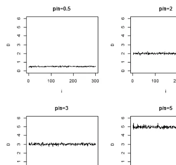
sample sizesn and diﬀerent dimensionspare generated from multivariate normal distributions. Without loss of generality, for each data set, the corresponding true covariance matrix is ap-dimensional symmetric matrix with 1 as diagonal values and 0.4 as oﬀ-diagonal values; and the true mean vectorµis generated fromN(0,0.01).

For each graph reported in this section (Figs. 1–4), the variable i in the x-axis ranges from 1 to 300. Eachicorresponds to data sets with dimensionpi and sample

size ni. Since p/n is a key value in studying the error patterns, in each graph of

Figs. 1–4, the relationship betweenpi andni is

pi ni

=c, (2.6)

where c is a fixed constant. That is, in each graph, the ratio between the dimen-sion and the sample size is fixed, with the dimendimen-sion and the sample size growing together. To be precise, in the four graphs of Fig. 1,nis are set as 28+2i,29+i,29+i

and 29 +i, respectively, and correspondingly,pis are 0.5(28 + 2i),2(29 +i),3(29 +i)

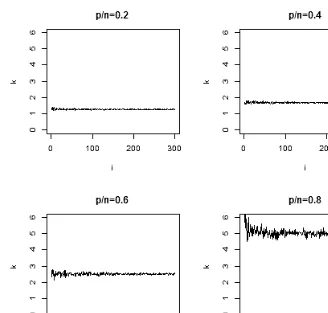
and 5(29 +i), which guarantees thatpi/ni is a fixed value. In Figs. 2–4,nis are all

set as 25 + 5i, andpis are 0.2(25 + 5i),0.4(25 + 5i),0.6(25 + 5i), and 0.8(25 + 5i).

(6)

Fig. 1. Diﬀerence between E( ˆP∗2

1 ) andP∗2. The mean eﬀect is measured by assuming that the true

covariance matrix is known. In each graph, the dimensionpand the sample sizengrow together with the same ratioi. The sample mean overestimatesP∗2_{and the diﬀerence}_D_{fluctuates around}

the value ofp/n.

2.1. Mean effect

To study the impact of the sample mean vector on the optimal expected gain/loss, assume that the true covariance matrix Σ is known. The impact of the sample mean can be measured by the diﬀerences ˆP∗2₋_P_ˆ∗2

2 or ˆP1∗2−P∗2. The results of such diﬀerences are summarized in the following theorem.

Theorem 2.1. Suppose that x= (x1, x2, . . . , xp)T,and xfollows a p-dimensional

multivariate normal distribution with mean µ and covariance matrix Σ. µˆ and S

are the sample mean and the sample covariance matrix, respectively. For a given

M, we have

E[ ˆP∗2−Pˆ2∗2|S=M] = 1

ntr[h(M

(7)

Fig. 2. Ratio between E( ˆP∗2

2 ) andP∗2. The covariance eﬀect is measured by assuming that the

true mean is known. In each graph, the dimensionpand the sample sizengrow together with the same ratioi. The overestimating ratio incurred by the sample covariance matrix is stable around a value related top/n.

and

E[ ˆP1∗2−P∗2] = 1

ntr[h(Σ

−1_{)Σ] =} p−1

n . (2.8)

Equivalently, ifΣis known,Pˆ2

1 −(p−1)/nis an unbiased estimator ofP∗2.

Proof. For multivariate normal distribution, Var(ˆµ) = E[ ˆµµˆT]−µµT. Moreover,

ˆ

µandS are independent. Therefore, we have

E[ ˆµTh(S−1) ˆµ|S] = E[tr( ˆµTh(S−1) ˆµ)|S]

= tr{E[ ˆµµˆT]h(S−1)}

= tr{[Var( ˆµ) +µµT]h(S−1)}

= tr

Σ

n +µµ

T _h₍_S−1₎

= 1

ntr[h(S

−1_{)Σ] +}

µTh(S−1)µ.

(8)

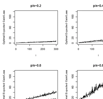
Fig. 3. Plug-in optimal expected gain/loss ˆP∗ _{versus benchmark value}_P∗_{. In each graph, the}

dimensionpand the sample sizengrow together with the same ratioi. Asp/ngrows larger, ˆP∗

deviates further fromP∗_.

According to (2.5), S is known to be the real covariance matrix Σ so that D = (p−1)/n. For detail, please refer toAnderson (2003). This gives (2.7). The proof of (2.8) is similar.

Simulation results are presented below. Define

D= E( ˆP1∗2)−P∗2. (2.10)

In the four graphs of Fig. 1, the y-axis measures the diﬀerence D and the x-axis denotes the variablei. For eachi, we simulate 30 data sets with the same covariance matrix and the same mean vector using a multivariate normal distribution. For each data set, we have a value ˆP∗2

1 . Then E( ˆP1∗2) is approximated by taking the sample average of these 30 values of ˆP∗2

(9)

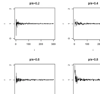
Fig. 4. Ratio between E( ˆP∗2₎₋_γ₍_p₋₁₎_/n _and_γP∗2_{. In each graph, the dimension} _p_{and the}

sample sizengrow together with the same ratioi. After considering both eﬀects of the sample mean and the sample covariance matrix, an unbiased estimator is achieved.

D fluctuates around the value of p/n. It is possible to obtain an asymptotically unbiased estimator ofP2 _{by correcting ˆ}_P∗2

1 with the termp/n.

2.2. Covariance effect

In this section,µis known and only the impact of the sample covariance matrix is

considered. Random matrix theory is employed to investigate the eﬀect ofS. The details are referred to Marˇcenko & Pastur (1967), Bai & Silverstein (2010), Bai

(1999),Baiet al.(2007).

Suppose that{zjk, j= 1, . . . , n, k= 1, . . . , p}is a set of double arrays ofi.i.d.real

random variables with mean 0 and varianceσ2_{. The empirical spectral distribution} of the sample covariance matrixT is defined as:

FT(x) = 1 p

p

i=1

(10)

whereλi is theith smallest eigenvalue ofT and

1(λi≤x) =

1 ifλi≤x,

0 otherwise. (2.12)

ByBai (1999), ifp/n→y ∈(0,∞), then with probability one,FT(x) converges to

the Marˇcenko–Pastur (M–P) lawFy(x) almost surely, where the M–P law is defined

as follows:

Definition 2.1 (Marˇcenko–Pastur Law,Marˇcenko & Pastur (1967)). The density function of the limit spectral distributionFy(x) is given by:

fy(x) =

  

 

1 2πxyσ2

(b−x)(x−a), ifa≤x≤b,

0, otherwise.

(2.13)

It has a point mass 1−1/y at the origin if y >1, where a= σ2₍₁₋√_y₎2_, _b ₌

σ2_{(1 +}√_y₎2_,_p/n_→_y_∈₍₀_,_∞_{). If}_σ2_{= 1, then it is called the standard M–P law.}

The bias of ˆP∗

2 in the estimation ofP∗ is explained in the following theorem. Theorem 2.2. Consider the notation in Theorem 2.1. Let Σn be the covariance

matrixΣof the firstp(n)stocks. Suppose that λmin(Σn),the smallest eigenvalue of

Σn is bounded below by a positive constant. Then,the ratio

k=E( ˆP ∗2 2 )

P∗2 →γ, (2.14)

where

γ= b

a

1

xdFy(x) =

1

1−y >1. (2.15)

Equivalently, ifµis known,Pˆ₂∗2/γ is an asymptotically unbiased estimator ofP∗2.

Proof. Applying Lemma A.2 and Lemma 3.1, part (b) ofBaiet al.(2009a), we see that

µTS−1µ µTΣ−1µ→

a.s._γ _and 1TS−11

1TΣ−1₁→

a.s._γ. _(2.16)

Note that|µTS−1µ/µTΣ−1µ|is bounded above by 1/λˆ1 where ˆλ1 is the smallest eigenvalue ofS. LetSn be the sample covariance matrixS obtained from the first n sample and the first p(n) stocks. It is obvious that thatSn is a principal

(11)

convergence. The desired results follow from the fact that

µTh(S−1)µ=µTS−1µ−(1TS−11)−1(µTS−1µ)2 (2.17)

and

µTh(Σ−1)µ=µTΣ−1µ−(1TΣ−11)−1(µTΣ−1µ)2. (2.18)

Below, simulation studies are conducted to give an intuitive feeling of the results in Theorem 2.2. In Fig. 2, they-axis measures the ratiokand thex-axis denotes the variable i. Again, for each i, 30 data sets are simulated using the same covariance matrix and the mean vector. For each data set, we have a value of ˆP∗2

2 , then E( ˆP2∗2) is approximated by taking the sample average of these 30 values of ˆP∗2

2 as the estimate of the mean. It is seen that for a fixedµ, the overestimating ratio incurred

byS is stable around the valueγ aspandnincrease withi.

2.3. Joint effect

To consider the joint eﬀect, we examine the sample mean and the sample covari-ance matrix simultaneously. The following theorem explains the bias of ˆP∗ _{in the} estimation ofP∗_.

Theorem 2.3. Consider the notation in Theorem 2.1. Let Σn be the covariance

matrix Σ of the first p(n) stocks. Denote by λmin(Σn) andλmax(Σn) the smallest

and greatest eigenvalue ofΣn respectively. Suppose that λmin(Σn)is bounded below

by a positive constant andλmax(Σn)is bounded above by another positive constant.

Assume that 1T_Σ−1₁₌_O₍_p_{). Then}_, _{the ratio}

r= E( ˆP

∗2₎₋_γ₍_p₋₁₎_/n

γP∗2 = 1. (2.19)

Equivalently, [ ˆP∗2₋_γ₍_p₋₁₎_/n_]_/γ _{is an asymptotically unbiased estimator of} _P∗2_.

Proof. LetT = Σ−1/2SΣ−1/2. Denote the smallest and greatest eigenvalues ofT

by ˜λ1 and ˜λp, respectively. Using Theorem 2.1,

E( ˆP∗2) = E( ˆP2∗2) + E( ˆP∗2−Pˆ2∗2)

= E( ˆP2∗2) +n−1Etr[h(S−1)Σ]

= E( ˆP2∗2) +n−1E[tr(T−1)]−E

n−11

T_Σ−1/2_T−2_Σ−1/2₁ 1TΣ−1/2_T−1_Σ−1/2₁

=E1+n−1E2+n−1E3.

E1/P2→γ according to Theorem 2.2.

The random matrix theory (Bai 1999) suggests that p−1_tr(_T−1_{) converges} almost surely to γ. The quantity tr(T−1_{) is bounded above by} _p/_˜_λ

(12)

apply the dominating convergence theorem, a lower bound of ˜λ1 is needed. To see this, let Sn be the sample covariance matrix S obtained from the first n sample

and the firstp(n) stocks. It is obvious that Sn is a principal sub-matrix of Sn+1.

Therefore, asnincreases, ˆλ1is monotonic decreasing and converges to a limit that is bounded below byaλmin(Σ). Consequently, a lower bound of ˜λ1 can be given by

aλmin(Σ)/λmax(Σ).

Next, we show thatE3 iso(p). Note that

1TΣ−1/2_T−2_Σ−1/2₁ 1T_Σ−1/2_T−1_Σ−1/2₁ ≤

˜

λp

˜

λ1

→ _ab. (2.20)

It can be checked that ˜λ1≥aλmin(Σ)/λmax(Σ) and ˜λp≤bλmax(Σ)/λmin(Σ). Then,

dominating convergence theorem can be used.

The plug-in optimal expected gain/loss ˆP∗ _{is plotted against the theoretical} value P∗_{. The solid line in Fig. 3 shows the behavior of ˆ}_P∗ _{and the dash line} denotesP∗_.

It is observed that as p/n grows larger, ˆP∗ _{deviates further from} _P∗_{. From} Theorem 2.3, consider the quantity

r=E( ˆP

∗2₎₋_γ₍_p₋₁₎_/n

γP∗2 . (2.21)

Since the ratio between E( ˆP∗2₎₋_γ₍_p₋₁₎_/n_and_γP∗2_{fluctuates around 1, the} value (E( ˆP∗2)−γ(p−1)/n)/γ is approximately the same asP∗2, see Fig. 4.

From these numerical studies, we see that both the sample mean and the sample covariance matrix over predict the optimal expected gain/loss. If we fix the sample covariance matrix as known, the effect of the sample mean onP∗2_{is additive; while if} the sample mean is fixed, the effect of the sample covariance matrix is multiplicative; if we take the two variables simultaneously, the effect can be eliminated by two steps. It can also be argued that the error patterns incurred by ˆµandS together cannot be ignored.

3. Shrinkage Estimator

(13)

3.1. Estimating the covariance matrix

The shrinkage covariance matrix is a linear combination of the sample covariance matrix and a highly structured covariance matrix, which is estimated from the data. The structured covariance matrix is also called the shrinkage target. The weight on the shrinkage target, which is called shrinkage intensity, is chosen based on the criterion of minimizing a risk function.

3.1.1. Shrinkage target

We use the largest eigenvalue of the sample covariance matrix to specify the shrink-age target, which is defined as:

F =λ1I, (3.1)

where λ1 denotes the largest eigenvalue of S. Then, the shrinkage covariance matrix is

S† ₌_αF_{+ (1}₋_α₎_S, _(3.2) where αis the shrinkage intensity. The shrinkage target chosen according to (3.1) guarantees that the greatest eigenvalue of S† _{does not depend on the shrinkage} intensityα. This means that the amount of information contained in the first prin-cipal component obtained byS† _{is not aﬀected by the shrinkage.}

3.1.2. Computation of the shrinkage intensity

Define F = (fij),S = (sij) and Σ = (σij). The shrinkage intensity is estimated by

minimizing the risk function, which is defined and decomposed as follows:

R(α) = E(L(α))

=

p

i=1

p

j=1

E[αfij+ (1−α)sij−σij]2

=

p

i=1

p

j=1

[α2E(fij−sij)2+ (1−2α)Var(sij) + 2αCov(fij, sij)]. (3.3)

Here, we have used

E(fij−sij)(sij−σij) = E(fij−σij)(sij−σij)−E(sij−σij)2

= Cov(fij, sij) + E(fij−σij)·E(sij−σij) + Var(sij)

= Cov(fij, sij) + Var(sij). (3.4)

Diﬀerentiating R(α) with respect to α, we obtain the estimate of the shrinkage intensityαas:

α∗₌ p

i=1 p

j=1Var(sij)− p

i=1 p

j=1Cov(fij, sij) p

i=1 p

j=1E(fij−sij)2

(14)

3.2. New estimator

From Sec. 2, it is known that E( ˆP∗2_{) is overestimated due to using the sample} mean ˆµand the sample covariance matrix S. To construct the new estimator, we

introduce Theorem 3.8beneath, using conditional expectations. Similar to Sec. 2, introduce the following notations:

ˆ

P†2₌_f_(ˆ

µ, S†) = ˆµTh((S†)−1) ˆµ (3.6)

and

ˆ

P₂†2=f(µ, S†) =µTh((S∗)−1))µ. (3.7)

The eﬀect ofµon ˆP†2is described in the following theorem.

Theorem 3.1. For a given M,

E[ ˆP†2−Pˆ2†2|S=M] = 1

nE[trh([αF + (1−α)M]

−1_)Σ]_. _(3.8)

Proof. Using the independence of ˆµandS, we have

E( ˆP†2_|_S₌_M_{) = E( ˆ}

µTh(S†−1) ˆµ|S=M)

= E[E( ˆµTh(S†−1) ˆµ|S=M)]

= 1

nE[trh(S

†−1_)Σ

|S=M] + E[µTh(S†−1)µ|S=M]. (3.9)

The following theorem further suggests that if Σ is known, asymptotically conservative estimator ofP∗ _{can be constructed for both}_y_∈₍₀_,_{1) and}_y _∈₍₁_,_∞₎ cases. In certain situations, underestimated estimators are less dangerous than over-estimated estimators. Note thatP is always positive. IfP∗_{is negative and the} cor-responding investment amount is ω∗, negating ω∗ always gives positive expected

gain/loss. Therefore, such a negative P∗ _{can never be optimal. If} _P∗2 _is overesti-mated, the computed minimal capital requirement may not be suﬃcient to protect a financial institution against the risk.

Theorem 3.2. For any given p-dimensional vector u,

E(uTh(Σ−1)u)≥E(uTh(Σ†−1)u), (3.10)

whereΣ†₌_αF _{+ (1}₋_α_)Σ.

Proof. See Appendices A and B.

Inspired by Theorem3.8, a new estimator is constructed below. DefineK as

K= 1

ntr[h(S

(15)

The new estimator ofP is given by ˆ P∗ new=      ˆ

µTh(S†−1) ˆµ−K, if ˆµTh(S†−1) ˆµ≥K,

ˆ

µTh(S†−1) ˆµ, otherwise.

(3.12)

When ˆµTh(S†−1) ˆµis smaller thanK, we can only use the shrinkage covariance

matrix. Although the eﬀect of the sample mean is not taken into account in this case, the estimator is at least better than the plug-in estimate. Moreover, ˆP∗

new is well-defined even when the sample covariance matrix is singular. In practice, Σ is unknown. Therefore, ˆP∗

newcan be biased. To mitigate the bias,αis chosen according to the method proposed in the next section.

3.3. Algorithm

3.3.1. Shrinkage intensityα∗

According to the shrinkage target,F =λ1I. Recall that the theoretical expression ofα∗ _is

α∗₌ p

i=1 p

j=1Var(sij)− p

i=1 p

j=1Cov(fij, sij) p

i=1 p

j=1E(fij−sij)2

. (3.13)

To estimateα∗_{, the values Var(}_s

ij), Cov(fij, sij) and E(fij−sij)2 need to be

esti-mated.

The bootstrap method (see, for example,Efron & Tibshirani (1993)) is chosen to give numerical estimates of these three values. In this paper,pis large relative to

n, in which case the sample covariance matrix S is singular. Since the parametric resampling needs the sample covariance matrix to be invertible, parametric resam-pling is inappropriate. Consequently, the nonparametric resamresam-pling method is used to generate diﬀerent data sets based on the observations.

Suppose that the number of resampling isN. Each time, resampling is taken within each asset with replacement. Fork∈ {1, . . . , N}, thekth data set is generated as follows:      

x(₁₁k) x(₁₂k) . . . x(₁k_p)

x(21k) x (k)

22 . . . x (k) 2p . . . .

x(nk1) x (k)

n2 . . . x (k)

np       ,

and thekth sample covariance matrixS(k) _is

     

s(11k) s (k)

12 . . . s (k) 1p s(21k) s

(k)

22 . . . s (k) 2p . . . .

s(pk1) s (k)

p2 . . . s (k)

(16)

Thekth shrinkage target is

F(k)=λ(1k)I, (3.14)

whereλ(1k)is the largest eigenvalue ofS(k). Then, we get the estimates of the three values as:

ˆ

Var(sij) =

1

N−1

N

k=1

(s(_ijk)−¯sij)2, (3.15)

ˆ

Cov(fij, sij) =

1

N−1

N

k=1

(s(_ijk)−¯sij)(fij(k)−f¯ij), (3.16)

ˆ

E(fij−sij)2 = 1 N

N

k=1

(fij(k)−s

(k)

ij )2, (3.17)

where ¯sij =Nk=1s (k)

ij /N and ¯fij=Nk=1f (k)

ij /N. The estimate ofα∗ is

ˆ

α∗₌ p

i=1 p

j=1Var(ˆ sij)−pi=1 p

j=1Cov(ˆ fij, sij)

p

i=1 p

j=1E(ˆ fij−sij)2

. (3.18)

To estimateK, for simplicity, we replace Σ by the sample covariance matrixSand define ˆK as

ˆ

K= 1

ntr[h(S

†−1₎_S_)]_. _(3.19)

3.4. Bias of the new estimator

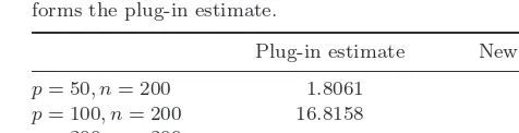
In this part, MSE of the new estimator is calculated using simulation studies and compared with plug-in estimate. For simplicity, the true mean vector is generated from N(0,1), and the true covariance matrix is a p-dimensional identity matrix. Four cases are considered, that is,p= 50, n= 200;p= 100, n= 200;p= 200, n= 200 and p= 400, n= 200. For each case, 100 data sets are generated. The results are shown in Table 1.

4. Simulation Study

(17)

Table 1. MSE of the new estimator. The MSE of the new esti-mator is compared with the plug-in estimate considering four combinations of diﬀerent dimension and diﬀerent sample size. The new estimator not only works whenp > n, but also outper-forms the plug-in estimate.

Plug-in estimate New estimator

p= 50, n= 200 1.8061 0.0954

p= 100, n= 200 16.8158 0.1595

p= 200, n= 200 — 1.8771

p= 400, n= 200 — 12.0717

4.1. Comparison

(1) Benchmark Value (rreal). The benchmark value is the theoretical optimal expected gain/loss computed using the true mean vectorµand the true

covari-ance matrix Σ of the data set.

(2) Plug-in Estimate (rplug). The plug-in estimate is computed using the sample mean vectorµˆand the sample covariance matrixS.

(3) Shrinkage Estimate(rshrink). The shrinkage estimate is computed by plugging in the sample meanµˆand the shrinkage covariance matrixS∗. Following Ledoit & Wolf (2004a), the shrinkage target is chosen as the constant correlation model, because it is easy to implement.

(4) Bootstrap Corrected Estimate(rbs). InBaiet al.(2009b), an eﬃcient estimator using the theory of random matrices was developed to solve the over prediction problem. A parametric bootstrap technique was employed in their study. The procedure is as follows:

(a) A resampleχ∗_{= (}_X∗

1, . . . , Xn∗) is drawn from thep-dimensional

multivari-ate normal distribution with mean vectorµˆ and covariance matrixS. (b) The sample mean vector and the sample covariance matrix of the resample

data set is denoted by µˆ_bs and Sbs, respectively. Then, by applying the optimization procedure again, we obtain the bootstrapped plug-in estimate of the optimal expected gain/lossr∗

plug.

(c) The bootstrapped corrected gain/loss estimate is given by:

rbs=rplug+ 1

√_γ(rplug−r∗plug). (4.1)

4.2. Constructing the data set

(18)

as the true parameters from which the empirical returns are generated using the multivariate normal distribution.

Since the market changes significantly across time, we fix the number of obser-vationsnas 50 days and 100 days. Therefore, we have six combinations ofpandn, namely p= 30, n= 50; p= 30, n= 100;p= 60, n= 50; p= 60, n= 100;p= 80, n= 50 andp= 80, n= 100, respectively.

4.3. Simulation results

For each case, we simulate 100 data sets and for each data seti, we calculate the values ofri

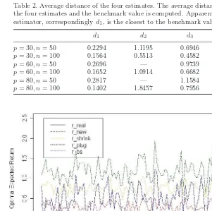
[image:18.595.77.378.262.561.2]

real, rinew, rplugi , rishrink and ribs. We use d1, d2, d3 and d4 to measure the

Table 2. Average distance of the four estimates. The average distance between the four estimates and the benchmark value is computed. Apparently, the new estimator, correspondinglyd1, is the closest to the benchmark value.

d1 d2 d3 d4

p= 30, n= 50 0.2294 1.1195 0.6946 0.4903 p= 30, n= 100 0.1564 0.5513 0.4582 0.2711

p= 60, n= 50 0.2696 — 0.9739 —

p= 60, n= 100 0.1652 1.0914 0.6682 0.4040

p= 80, n= 50 0.2817 — 1.1584 —

[image:18.595.83.372.264.344.2]

p= 80, n= 100 0.1402 1.8457 0.7956 0.5714

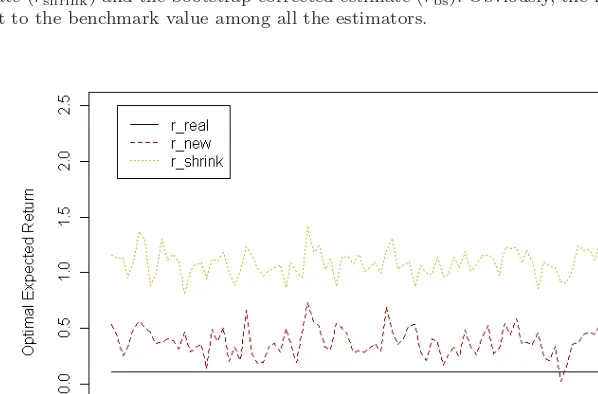
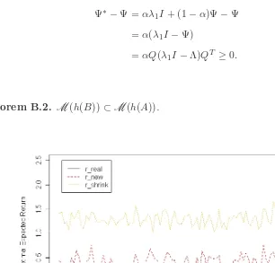
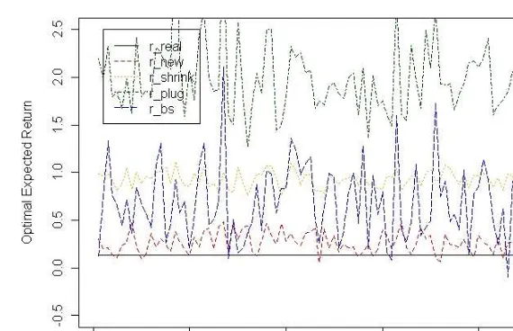
Fig. 5. Model comparison p = 30, n = 50. The new estimator (rnew) of the optimal expected

gain/loss is compared with the benchmark value (rreal), the plug-in estimate (rplug), the shrinkage

estimate (rshrink) and the bootstrap corrected estimate (rbs). Obviously, the new estimator is the

(19)

[image:19.595.78.377.61.257.2]

Fig. 6. Model comparisonp = 30, n = 100. The new estimator (rnew) of the optimal expected

closest to the benchmark value among all the estimators.

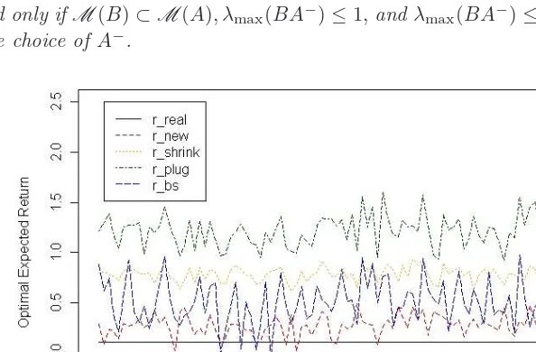
Fig. 7. Model comparison p = 60, n = 50. The new estimator (rnew) of the optimal expected

[image:19.595.78.377.333.530.2]

(20)

average distance between the four estimates and the benchmark value. Define

d1 = 1 100

100

i=1

|rinew−rireal|, d2= 1 100

100

i=1

|rplugi −rireal|,

d3 = 1 100

100

i=1

|rishrink−rreali |, d4= 1 100

100

i=1

|ribs−rireal|.

From Table 2, observe thatrnewstill has the minimum average distance among all the estimators. When the sample covariance matrix is not singular, rbs is the second best estimator, andrshrink becomes worse asp/ngrows larger. Figures 5–7, A.1, B.1 and B.2 also demonstrate the above conclusion. Moreover, rnew is much more stable than the other estimators.

5. Conclusion

In this study, we proposed a new estimator for evaluating the optimal expected gain/loss of a large dimensional portfolio.

In the MV portfolio optimization procedure, it is well known that the plug-in optimal expected gain/loss is not a good estimator since using the sample mean and the sample covariance matrix of the historical data incurs substantial errors. Instead of constructing new estimators of the mean and the covariance matrix, this paper incorporates the interaction eﬀect of these two quantities and explores how the sample mean and the sample covariance matrix behave based on the idea of conditional expectation.

It is found that the eﬀect of the sample mean is additive and the eﬀect of the sample covariance matrix is multiplicative. Both of them over-predict the optimal expected gain/loss. In the financial market, the number of stocks can be very large while the sample size is usually moderate. Therefore, p/n can be substantial and in such a case the sample covariance matrix tends to be singular. This paper used the shrinkage methods to construct a stable covariance matrix which was invertible for both p < n and p ≥ n. Matrix inequalities were employed to prove that the shrinkage covariance matrix led to an estimate of the optimal expected gain/loss which was smaller than the plug-in estimate and closer to the benchmark value. Simulation studies show that the new estimator has better performance than the previous methods.

Acknowledgments

(21)

HKSAR-RGC-CRF No. CityU8/CRG/12G (N.H. Chan), and the National Research Foundation of Korea (NRF) of the government of Korea (MSIP) No. 2011-0030810 (C.T. Ng).

Appendix A. Preliminaries

Definition A.1. The Loewner partial ordering on the set of positive semidefinite matricesGis defined as follows: forA, B∈G, A≤B iﬀB−A∈G.

Theorem A.1. If A and B are positive definite Hermitian matrices, then A ≥ B⇔B−1_≥_A−1_.

Theorem A.2. A and B are n ×n Hermitian matrices.A >0 andB >0, then

A≥B⇔λmax(BA−1₎_≤₁_.

Theorem A.3. If A ≥ B ≥ 0, then M₍_B₎ _⊂ M₍_A₎_, _where M₍_A₎ _{denotes the}

column space of A.

Theorem A.4. If A and B are positive semidefinite Hermitian matrices, then

A≥B⇔M₍_B₎_⊂M₍_A₎_{, and A}₍_A₋_B₎_A_≥₀_.

Theorem A.5. A and B are Hermitian matrices,and A≥0,B≥0. Then A≥B if and only ifM₍_B₎_⊂M₍_A₎_{, λ}_max(_BA−₎_≤₁_,_and_λ_max(_BA−₎_≤₁_{is independent} of the choice ofA−_.

Fig. A.1. Model comparisonp= 60, n= 100. The new estimator (rnew) of the optimal expected

(22)

Theorem A.6. If B = 0,then B′_A−_B _{is independent of the choice of} _A− _{if and} only ifM₍_B₎_⊂M₍_A_).

Appendix B. Proof of Theorem 3.2

Let Ψ be a positive definite matrix, λ1 be the greatest eigenvalue of Ψ, Ψ† =

αλ1I+ (1−α)Ψ], A = Ψ−1, and B = Ψ†−1. To prove Theorem 3.2, we have to prove the following theorems first.

Theorem B.1. A≥B.

Proof. By TheoremA.1, Ψ−1 _≥_Ψ†−1 _⇔_Ψ† _≥_{Ψ. Factorize Ψ as} _Q_Λ_QT_{, where} QQT ₌_I_{, Λ = diag(}_λ

1, λ2, . . . , λp).

Ψ∗−Ψ =αλ1I+ (1−α)Ψ−Ψ

=α(λ1I−Ψ)

=αQ(λ1I−Λ)QT ≥0. (B.1)

Theorem B.2. M₍_h₍_B₎₎_⊂M₍_h₍_A_)).

Fig. B.1. Model comparisonp = 80, n= 50. The new estimator (rnew) of the optimal expected

(23)

Fig. B.2. Model comparisonp= 80, n= 100. The new estimator (rnew) of the optimal expected

closest to the benchmark value among all the estimators.

Proof. If we can find a matrix X which makesh(B) =h(A)X hold, then we can obtain the result. Let

X =A−1

I−B11

T

1T_B₁

B, (B.2)

then,

h(A)X =

A−A11

T_A

1T_A₁

A−1

I−B11

T

1T_B₁

B

=

I−A11

T

1TA1 I−

B11T 1TB1

B

=

I−B11

T

1T_B₁

B=h(B), (B.3)

the proof is completed.

Theorem B.3. h(A)≥h(B).

Proof. According to Theorem A.4 and Theorem B.2, it is equivalent to proving that when M₍_h₍_B₎₎_⊂M₍_h₍_A_{)) holds,}

h(A)≥h(B)⇔λ1[h(B)h(A)−_]_≤₁_, _(B.4) where h(A)− _{can be any general inverse of}_h₍_A_{). From Theorem A.4, the problem} converts to prove that whenM₍_h₍_B₎₎_⊂M₍_h₍_A_{)) holds,}

(24)

Do full rank decomposition toh(A), so thath(A) =LL∗_{. Then}

h(A)[h(A)−h(B)]h(A)⇔L∗(h(A)−h(B))L≥0. (B.6)

Multiply (L∗_L₎−1_{on both sides of}_L∗₍_h₍_A₎₋_h₍_B₎₎_L_{, and we get}

L∗(h(A)−h(B))L⇔I−T∗h(B)T ≥0

⇔λ1(T∗h(B)T)≤1

⇔λ1(h(B)T T∗)≤1

⇔[λ1[h(B)h(A)+]≤1, (B.7)

whereT =L(L∗_L₎−1 _and_{T T}∗₌_L₍_L∗_L₎−2_L∗₌_h₍_A₎+_. From TheoremA.6, whenM₍_h₍_B₎₎_⊂M₍_h₍_A_{)) holds,}

λ1[h(B)h(A)+] =λ1[h(B)h(A)−_]_, _(B.8)

where h(A)− _{can be any general inverse of} _h₍_A_{). One of the general inverses of}

h(A) is

h(A)−₌

I−11

T_A

1TA1

A−1. (B.9)

λ1[(h(B)h(A)−_{)] =}_λ 1

B

I−11

T_B

1TB1 I− 11T_A 1TA1

A−1

=λ1

B

I−11

T_B

1T_B₁

A−1

=λ1

A−1B

I−11

T_B

1TB1

≤λ1(A−1B)λmax

I−11

T_B

1TB1

=λ1(BA−1)λmax

I−11

T_B

1T_B₁

. (B.10)

SinceA≥B, by Theorem A.2,λ1(BA−1₎_≤_1._I₋11T_B

1TB1 is an idempotent matrix,

therefore, the largest eigenvalue of it is 1. Thus we have

h(A)≥h(B). (B.11)

Left and right multiply h(A)− h(B) by µT and µ, respectively.

(25)

References

T. W. Anderson (2003)An Introduction to Multivariate Statistical Analysis, third edition. New York: Wiley.

Z. Bai (1999) Methodologies in spectral analysis of large dimensional random matrices, a review,Statistica Sinica16_{(1), 611–677.}

Z. Bai, H. Liu & W. K. Wong (2009a) Enhancement of the applicability of Markowitz’s portfolio optimization by utilizing random matrix theory, Mathematical Finance 19_{(4), 639–667.}

Z. Bai, H. Liu & W. K. Wong (2009b) On the Markowitz mean-variance analysis of self-financing portfolios,Risk and Decision Analysis1_{, 35–42.}

Z. Bai & J. W. Silverstein (2010)Spectral Analysis of Large Dimensional Random Matrices, second edition. New York: Springer.

Z. Bai, B. Q. Miao & G. M. Pan (2007) On asymptotics of eigenvectors of large sample covariance matrix,Annals of Probability35_{(4), 1532–1572.}

S. J. Brown (1976) Optimal Portfolio Choice Under Uncertainty: A Bayesian Approach. PhD Thesis, University of Chicago, 1976.

B. F. Efron & R. J. Tibshirani (1993)An Introduction to the Bootstrap. London: Chapman and Hall.

G. M. Frankfurter, H. E. Phillips & J. P. Seagle (1971) The eﬀects of uncertain means, variances, and covariances, Journal of Financial and Quantitative Analysis 6 _(5),

1251–1262.

P. A. Frost & J. E. Savarino (1986) An empirical bayes approach to eﬃcient portfolio selection,Journal of Financial and Quantitative Analysis21_{(3), 293–305.}

W. James & C. M. Stein (1961) Estimation with quadratic loss,Proceedings of the Fourth Berkeley Symposium on Mathematical Statistics and Probability1, 361–380. P. Jorion (1986) Bayes-stein estimation for portfolio analysis, Journal of Financial and

Quantitative Analysis21_{(3), 279–292.}

B. Korkie & H. J. Turtle (2002) A mean-variance analysis of self-financing portfolios,

Management Science48_{(3), 427–443.}

O. Ledoit & M. Wolf (2003) Improved estimation of the covariance matrix of stock returns with an application to portfolio selection,Journal of Empirical Finance10_{, 603–621.}

O. Ledoit & M. Wolf (2004a) Honey, I shrunk the sample covariance matrix, Portfolio Management31_{(4), 110–119.}

O. Ledoit & M. Wolf (2004b) A well-conditioned estimator for large-dimensional covariance matrices,Journal of Multivariate Analysis88_{, 365–411.}

V. A. Marˇcenko & L. A. Pastur (1967) Distribution of eigenvalues for some sets of random matrices,Mathematics of the USSR-Sbornik1_{(4), 457–483.}

H. Markowitz (1952) Portfolio selection,Journal of Finance7_{(1), 77–91.}