www.elsevier.com/locate/cor
Biclustering in data mining
Stanislav Busygin
a, Oleg Prokopyev
b,∗, Panos M. Pardalos
aaDepartment of Industrial and Systems Engineering, University of Florida, Gainesville, FL 32611, USA bDepartment of Industrial Engineering, University of Pittsburgh, Pittsburgh, PA 15261, USA
Available online 6 February 2007
Abstract
Biclustering consists in simultaneous partitioning of the set of samples and the set of their attributes (features) into subsets (classes). Samples and features classified together are supposed to have a high relevance to each other. In this paper we review the most widely used and successful biclustering techniques and their related applications. This survey is written from a theoretical viewpoint emphasizing mathematical concepts that can be met in existing biclustering techniques.
䉷2007 Published by Elsevier Ltd.
Keywords:Data mining; Biclustering; Classification; Clustering; Survey
1. The main concept
Due to recent technological advances in such areas as IT and biomedicine, the researchers face ever-increasing challenges in extracting relevant information from the enormous volumes of available data[1]. The so-calleddata avalancheis created by the fact that there is no concise set of parameters that can fully describe a state of real-world complex systems studied nowadays by biologists, ecologists, sociologists, economists, etc. On the other hand, modern computers and other equipment are able to produce and store virtually unlimited data sets characterizing a complex system, and with the help of available computational power there is a great potential for significant advances in both theoretical and applied research. That is why in recent years there has been a dramatic increase in the interest in sophisticated data miningandmachine learning techniques, utilizing not only statistical methods, but also a wide spectrum of computational methods associated with large-scale optimization, including algebraic methods and neural networks.
The problems of partitioning objects into a number of groups can be met in many areas. For instance, the vector partition problem, which consists in partitioning ofn d-dimensional vectors intopparts has broad expressive power and arises in a variety of applications ranging from economics to symbolic computation (see, e.g.,[2–4]). However, the most abundant area for the partitioning problems is definitely data mining. Data mining is a broad area covering a variety of methodologies for analyzing and modeling large data sets. Generally speaking, it aims at revealing a genuine similarity in data profiles while discarding the diversity irrelevant to a particular investigated phenomenon. To analyze patterns existing in data, it is often desirable to partition the data samples according to some similarity criteria. This task is calledclustering. There are many clustering techniques designed for a variety of data types—homogeneous and
∗Corresponding author.
E-mail addresses:[email protected](S. Busygin),[email protected](O. Prokopyev),[email protected](P.M. Pardalos). 0305-0548/$ - see front matter䉷2007 Published by Elsevier Ltd.
nonhomogeneous numerical data, categorical data, 0–1 data. Among them one should mention hierarchical clustering [5],k-means[6], self-organizing maps (SOM)[7], support vector machines (SVM)[8,9], logical analysis of data (LAD) [10,11], etc. A recent survey on clustering methods can be found in[12].
However, working with a data set, there is always a possibility to analyze not only properties of samples, but also of their components (usually calledattributesorfeatures). It is natural to expect that each associated part of samples recognized as a cluster is induced by properties of a certain subset of features. With respect to these properties we can form an associated cluster of features and bind it to the cluster of samples. Such a pair is called abiclusterand the problem of partitioning a data set into biclusters is called abiclusteringproblem.
In this paper we review the most widely used and successful biclustering techniques and their related applications. Previously, there were published few surveys on biclustering[13,14], as well as a Wikipedia article[15]. However, we tried to write this survey from a more theoretical viewpoint emphasizing mathematical concepts that can be found in existing biclustering techniques. In addition this survey discusses recent developments not included in the previous surveys and includes references to public domain software available for some of the methods and most widely used benchmarks data sets.
2. Formal setup
Let a data set ofnsamples andmfeatures be given as a rectangular matrixA=(aij)m×n, where the valueaij is the expression ofith feature injth sample. We consider classification of the samples into classes
S1,S2, . . . ,Sr, Sk⊆ {1, . . . , n}, k=1, . . . , r, S1∪S2∪ · · · ∪Sr = {1, . . . , n},
Sk∩Sℓ= ∅, k, ℓ=1, . . . , r, k=ℓ.
This classification should be done so that samples from the same class share certain common properties. Correspond-ingly, a featureimay be assigned to one of the feature classes
F1,F2, . . . ,Fr, Fk ⊆ {1, . . . , m}, k=1, . . . , r, F1∪F2∪ · · · ∪Fr= {1, . . . , m},
Fk∩Fℓ= ∅, k, ℓ=1, . . . , r, k=ℓ,
in such a way that features of the classFkare “responsible” for creating the class of samplesSk. Such a simultaneous
classification of samples and features is calledbiclustering(orco-clustering).
Definition 1. A biclustering of a data set is a collection of pairs of sample and feature subsets B=((S1,F1)
(S2,F2), . . . , (Sr,Fr))such that the collection(S1,S2, . . . ,Sr)forms a partition of the set of samples, and the
collection(F1,F2, . . . ,Fr)forms a partition of the set of features. A pair(Sk,Fk)will be called abicluster.
It is important to note here that in some of the biclustering methodologies a direct one to one correspondence between classes of samples and classes of features is not required. Moreover, the number of sample and feature classes is allowed to be different. This way we may consider not only pairs(Sk,Fk), but also other pairs(Sk,Fℓ),k=ℓ. Such pairs
will be referred to asco-clusters. Another possible generalization is to allowoverlappingof co-clusters.
The criteria used to relate clusters of samples and clusters of features may have different nature. Most commonly, it is required that the submatrix corresponding to a bicluster either is overexpressed (i.e., mostly includes values above average), or has a lower variance than the whole data set, but in general, biclustering may rely on any kind of common patterns among elements of a bicluster.
3. Visualization of biclustering
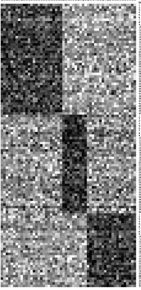
Fig. 1. Partitioning of samples and features into three clusters.
When one constructs a reasonable biclustering of a data set and then reorders samples and features by cluster numbers, the heatmap is supposed to show a “checkerboard” pattern as diagonal blocks show biclusters that are the distinguished submatrices according to the used biclustering method. Fig. 1 is an example of data set with three biclusters of overexpressed values visualized as the heatmap (in the black-and-white diagram darker pixels correspond to higher values).
4. Relation to SVD
Singular value decomposition(SVD) is a remarkable matrix factorization which generalizes eigendecomposition
of a symmetric matrix providing the orthogonal basis of eigenvectors. SVD is applicable to any rectangular matrix
A=(aij)m×n. It delivers orthogonal matricesU=(uik)m×pandV =(vj k)n×p(i.e., the columns of the matrices are
orthogonal to each other and have the unit length) such that
UTAV =diag(1, . . . ,p), p=min(m, n). (1)
The numbers12· · ·p0 are calledsingular values, the columns ofUare calledleft singular vectorsand
the columns ofVare calledright singular vectorsofA. This way, left singular vectors provide an orthonormal basis for columns ofA, and right singular vectors provide an orthonormal basis for rows ofA. Moreover, these bases are coupled so that
Avk=kuk,
ATuk=kvk,
whereuk is kth left singular vector, and vk iskth right singular vector of the matrix. The singular values ofA are
precisely the lengths of the semi-axes of the hyperellipsoidE= {Ax : x2=1}.
The SVD provides significant information about properties of the matrix. In particular, ifr is the last nonzero
singular value (i.e.,r+1= · · · =p=0), then
rank(A)=r,
null(A)=span{vr+1, . . . , vn}, ran(A)=span{u1, . . . , ur},
where span{x1, . . . , xk}denotes the linear subspace spanned by the vectorsx1, . . . , xk, null(A)= {x :Ax=0}is the
nullspace of the matrix, and ran(A)is the linear subspace spanned by the columns ofA. It is easy to see from these properties that the SVD is a very useful tool for dimensionality reduction in data mining. Taking also into account that the Frobenius norm of the matrix
one can obtain the best in sense of Frobenius norm low-rank approximation of the matrix by equating all singular values after someℓto zero and considering
˜
Such a low-rank approximation may be found inprincipal component analysis(PCA) withℓfirst principal components considered. PCA applies SVD to the data matrix after certain preprocessing (centralization or standardization of data samples) is performed. We refer the reader to a linear algebra text[17]for more theoretical consideration of the SVD properties and algorithms.
One may relate biclustering to the SVD via consideration an idealized data matrix. If the data matrix has a block-diagonal structure (with all elements outside the blocks equal to zero),it is natural to associate each block with a bicluster. On the other hand, it is easy to see that each pair of singular vectors will designate one such bicluster by nonzero components in the vector. More precisely, if the data matrix is of the form
A=
occupied byAk. In a less idealized case, when the elements outside the diagonal blocks are not necessarily zeros but
diagonal blocks still contain dominating values,the SVD is able to reveal the biclusters too as dominating components in the singular vector pairs.
Hence, the SVD represents a handy tool for biclustering algorithms. Below we show that many biclustering methods either use the SVD directly or have a certain association with the SVD concept. Furthermore, we believe that the introduction into SVD must precede any discussion on biclustering methods because its theoretical value for simul-taneous analysis of samples and features of data cannot be overestimated. As of now, not many biclustering methods are theoretically justified in sense that it is not clear what mathematical properties of sample/feature vectors would tie them together in a common bicluster in one or another biclustering routine. Next, it is not obvious whether results of two arbitrarily chosen biclustering methods applied to the same data matrix are expected to contradict each other or not, and, if the contradiction occurs, whether it is natural (e.g., two methods analyze completely different properties of data) or tells us that one method is more precise than the other. We see SVD as the tool for resolution of such issues as we may hope to bring biclustering to the common ground, for example, by relating each biclustering method to SVD after a certain algebraic transformation applied to the data.
5. Methods
5.1. “Direct clustering”
Apparently the earliest biclustering algorithm that may be found in the literature is so-called direct clustering by Hartigan[18]also known asblock clustering. This approach relies on statistical analysis of submatrices to form the biclusters. Namely, the quality of a bicluster(Sk,Fk)is assessed by the variance
VAR(Sk,Fk)=
i∈Fk
j∈Sk
(aij−k)2,
wherekis the average value in the bicluster:
k=
i∈Fk j∈Skaij |FkSk| .
A bicluster is considered perfect if it has zero variance, so biclusters with lower variance are considered to be better than biclusters with higher variance. This, however, leads to an undesirable effect: single-row, single-column submatrices become ideal biclusters as their variance is zero. The issue is resolved by fixing the number of biclusters and minimizing the objective
VAR(S,F)=
r
k=1
i∈Fk
j∈Sk
(aij−k)2.
Hartigan mentioned that other objective functions may be used to find biclusters with other desirable properties, e.g., minimizing variance in rows, variance in columns, or biclusters following certain patterns.
5.2. Node-deletion algorithm
A more sophisticated criterion for constructing patterned biclusters was introduced by Cheng and Church[19]. It is based on minimization of so-calledmean squared residue. To formulate it, let us introduce the following notation. Let
(r)ik = 1 |Sk|
j∈Sk
aij (2)
be the mean of theith row in the sample clusterSk,
(c)j k = 1 |Fk|
i∈Fk
be the mean of thejth column in the feature clusterFk, and
k=
i∈Fk j∈Skaij |FkSk|
be the mean value in the bicluster(Sk,Fk). Theresidueof elementaij is defined as
rij=aij−(r)ik − (c)
j k +k, (4)
i∈Fk,j ∈Sk. Finally, themean squared residuescore of the bicluster(Sk,Fk)is defined as
Hk=
i∈Fk
j∈Sk
(rij)2.
This value is equal to zero if all columns of the bicluster are equal to each other (that would imply that all rows are equal too). A bicluster(Sk,Fk)is called a-bicluster ifHk. Cheng and Church proved that finding the largest
square-bicluster isNP-hard. So, they used a greedy procedure starting from the entire data matrix and successively removing columns or rows contributing most to the mean squared residue score. The brute-force deletion algorithm testing the deletion of each row and column would be still quite expensive in the sense of time complexity as it would requireO((m+n)mn)operations. However, the authors employed a simplified search for columns and rows to delete choosing a column with maximal
d(j )= 1 |Fk|
i∈Fk
rij2,
a row with maximal
d(i)= 1 |Sk|
j∈Sk
rij2,
or subsets of columns or rows for whichd(j )ord(i)exceeds a certain threshold above the current mean square residue of the bicluster. They have proved that any such deletion can only decrease the current mean square residue. These deletions are performed until a-bicluster is obtained. Then, as the constructed co-cluster can be not maximal (i.e., some of the previously removed columns or rows can be added without violating the-bicluster condition), the authors used a column and row addition algorithm. Namely, they proved that adding any column (row) withd(j )(d(i)) below the current mean square residue does not increase it. Therefore, successive addition of such columns and rows leads to a maximal-bicluster.
Software implementation of the method as well as some test data sets are available at[20].
Bryan et al. improved the node-deletion algorithm of Cheng and Church applying a simulated annealing technique. They reported a better performance on a variety of data sets in[21].
5.3. FLOC algorithm
Yang et al. generalized the definition of residue used in the node-deletion algorithm to allow missing data entries (i.e., someaij may be unknown)[22,23]. For a bicluster(Sk,Fk), they introduced the notion ofalpha-occupancy meaning that for each samplej ∈Skthe number of known data entriesaij,i∈Fkis greater than|Fk|and for each
featurei∈Fkthe number of known data entriesaij,j ∈Sk is greater than|Sk|. They also defined thevolumeof
When no further residue reduction is possible, the method stops. It is easy to show that the computational complexity of the method isO((m+n)mnrp), wherepis the number of iterations till termination. The authors claim that in the computational experiments they performedpis of the order of 10.
The FLOC algorithm is also able to take into account various additional constraints on biclusters by eliminating certain feature/sample additions/removals from consideration.
5.4. Biclustering via spectral bipartite graph partitioning
In[24]Dhillon proposed the following method of biclustering. Represent each sample and each feature of a data set as a vertex of a graphG(V , E),|V| =m+n. Between the vertex corresponding to samplej=1, . . . , nand the vertex corresponding to featurei=1, . . . , mintroduce an edge with weightaij. The graph has no edges between vertices representing samples, as well as between vertices representing features. Thus, the graph is bipartite withFandS
representing its color classes. The graphGhas the following weighted adjacency matrix
M=
0 A
AT 0
. (5)
Now, a partition of the set of vertices intorpartsV1, V2, . . . , Vr,
V =V1∪V2∪ · · · ∪Vr,
Vk∩Vℓ= ∅, k=ℓ, k, ℓ=1, . . . , r,
will provide a biclustering of the data set. Define the cost of the partition as the total weight of edges cut by it:
cut(V1, . . . , Vr)= r−1
k=1
r
ℓ=k+1
i∈Vk
j∈Vℓ
mij. (6)
When we are looking for a biclustering maximizing in-class expression values (thus creating dominating submatrices of biclusters) it is natural to seek minimization of the defined cut value. Besides, we should be looking for rather balanced in size biclusters as otherwise the cut value is most probably minimized with all but one biclusters containing one sample-feature pair only. This problem can be tackled with an SVD-related algorithm. Let us introduce the following:
Definition 2. The Laplacian matrixLGofG(V , E)is a|V| × |V|symmetric matrix, with one row and one column
for each vertex, such that
Lij= ⎧ ⎨
⎩
kmik if i=j,
−mij if i=j and (i, j )∈E,
0, otherwise.
Let a partitionV =V1∪V2of the graph be defined via a±1 vectorp=(pi)i=1,...,|V|such that
pi=
+1, i∈V
1,
−1, i∈V2.
The Laplacian matrix is connected to the weight of a cut through the following:
Theorem 1. Given the Laplacian matrixLGof G and a partition vector p,the Rayleigh Quotient
pTLp pTp =
4
|V|cut(V1, V2).
By this theorem, the cut is obviously minimized with the trivial solution, i.e., when allpiare either−1 or 1. So, to
i∈V, and letW=diag(w1, w2, . . . , w|V|)be the diagonal matrix of these weights. We denote
weight(Vℓ)=
i∈Vℓ
wi.
Now, the following objective function allows us to achieve balanced clusters:
Q(V1, V2)=
Let us denoteℓ= i∈Vℓwi and introduce the generalized partition vector with elements
qi=
Minimizing expression (7) isNP-hard. However, a relaxed version of this problem can be solved via a generalized eigendecomposition (notice thatqTW e=0).
Theorem 3. The problem
is solved when q is the eigenvector corresponding to the second smallest eigenvalue2of the generalized eigenvalue
problem
Lz=W z. (9)
or denotingu=D11/2xandv=D12/2y,
D1−1/2AD2−1/2v=(1−)u,
D2−1/2ATD1−1/2u=(1−)v,
which precisely defines the SVD of the normalized matrix Aˆ =D1−1/2AD−21/2. So, the balanced cut minimization problem can be solved by finding the second largest singular value of this normalized matrix and the singular vector pair corresponding to it that can be used to obtain the biclustering to two classes. In case of multiclass partitioning, Dhillon usedℓ= ⌈log2r⌉singular vectorsu2, u3, . . . , uℓ+1andv2, v3, . . . , vℓ+1to form theℓ-dimensional data set rows of the matrixZ(which represent both samples and features of the original data set) are clustered with a simple
k-means algorithm[6].
Dhillon reports encouraging computational results for text mining problems. Very similar spectral biclustering routines for microarray data have been suggested by Kluger et al.[25]. In addition to working with the singular vectors ofAˆ, they considered two other normalization methods that can be used before applying the SVD. The first one is
bistochastization. It makes all row sums equal and all column sums equal too (generally, to a different constant). It is known from Sinkhorn’s theorem that under quite general conditions on the matrixAthere exist diagonal matricesD1
andD2such thatD1AD2achieves bistochastization[26]. The other approach is applicable if sample/feature subvectors within a bicluster are expected to be shifted by a constant with respect to each other (i.e., vectorsaandbare considered similar ifa≈b+e, whereis the constant andeis the all-one vector). When similar data are expected to be scaled by different constants (i.e.,a≈b), the desirable property can be achieved by applying a logarithm to all data entries. Then, defining
After computing the singular vectors, it is decided which of them contain the relevant information about the optimal data partition. To extract partitioning information from the system of singular vectors, each of them is examined by fitting to a piecewise constant vector. That is, the entries of an eigenvector is sorted and all possible thresholds between classes are considered. Such a procedure is equivalent to searching for good optima in one-dimensional k-means problem. Then few best singular vectors can be selected to runk-means on the data projected onto them.
5.5. Matrix iteration algorithms for minimizing sum-squared residue
but considers all the submatrices formed by them. The algorithm is based on algebraic properties of the matrix of residues.
For a given clustering of features(F1,F2, . . . ,Fq), introduce a feature cluster indicator matrix F =(fik)m×q
such thatfik= |Fk|−1/2ifi∈Fkandfik=0 otherwise. Also, for a given clustering of samples(S1,S2, . . . ,Sr),
introduce a sample cluster indicator matrixS=(sj k)n×r such thatsj k = |Sk|−1/2ifj ∈Skandsj k=0 otherwise.
Notice that these matrices are orthonormal, that is, all columns are orthogonal to each other and have unit length. Now, letH=(hij)m×nbe the residue matrix. There are two choices forhijdefinition. It may be defined similar to (4):
hij =aij−(r)ik −(c)j ℓ +kℓ, (10)
wherei∈Fℓ,j ∈Sk,(r)and(c)are defined as in (2) and (3), and
kℓis the average of the co-cluster(Sk,Fℓ):
kℓ= i∈Fℓ j∈Skaij |FℓSk| .
Alternatively,hij may be defined just as the difference betweenaij and the co-cluster average:
hij =aij−kℓ. (11)
By direct algebraic manipulations it can be shown that
H=A−F FTASST (12)
in case of (11) and
H=(I−F FT)A(I−SST) (13)
in case of (10).
The method tries to minimizeH2using an iterative process such that on each iteration a current co-clustering is updated so thatH2, at least, does not increase. The authors point out that finding the global minimum forH2over all possible co-clusterings would lead to anNP-hard problem. There are two types of clustering updates used: batch (when all samples or features may be moved between clusters at one time) and incremental (one sample or one feature is moved at a time). In case of (11) the batch algorithm works as follows:
Algorithm 1(CoclusH1).
Input:data matrix A,number of sample clusters r,number of feature clusters q. Output:clustering indicators S and F.
1.Initialize S and F.
2.obj val:= A−F FTASST2. 3. :=1,:=10−2A2{Adj ust able}. 4.While >:
4.1.AS:=F FTAS;
4.2.forj :=1to n assign jth sample to clusterSkwith smallestA·j− |Sk|−1/2AS
·k2; 4.3.update S with respect to the new clustering;
4.4.AF :=FTASST;
4.5.fori:=1to m assign ith feature to clusterFk with smallestAi·− |Fk|−1/2AF
k·2;
4.6.update F with respect to the new clustering; 4.7.oldobj :=obj val,obj val:= A−F FTASST2; 4.8. := |oldobj −obj val|.
In case of (10) the algorithm is similar but uses a bit different matrix manipulations:
Algorithm 2(CoclusH2).
Input:data matrix A,number of sample clusters r,number of feature clusters q. Output:clustering indicators S and F.
1.Initialize S and F.
2.obj val:= (I−F FT)A(I−SST)2. 3. :=1,:=10−2A2{Adj ust able}. 4.While >:
4.1.AS :=(I−F FT)AS,AP :=(I−F FT)A;
4.2.forj :=1to n assign jth sample to clusterSkwith smallestAP
·j− |Sk|−1
/2AS
·k2; 4.3.update S with respect to the new clustering;
4.4.AF :=FTA(I−SST),AP :=A(I−SST);
4.5.fori:=1to m assign ith feature to clusterFkwith smallestAP
i· − |Fk|−1/2AFk·2;
4.6.update F with respect to the new clustering;
4.7.oldobj :=obj val,obj val:= (I−F FT)A(I−SST)2; 4.8. := |oldobj−obj val|.
5.STOP.
To describe the incremental algorithm, we first note that in case of (10)His defined as in (13), and minimization ofH2is equivalent to maximization ofFTAS2. So, suppose we would like to improve the objective function by moving a sample from clusterSk to clusterSk′. DenoteFTAbyA¯ and the new sample clustering indicator matrix
byS˜. AsSandS˜differ only in columnskandk′, the objective can be rewritten as
¯AS˜·k′2− ¯AS·k′2+ ¯AS˜·k2− ¯AS·k2. (14)
So, the inner loop of the incremental algorithm looks through all possible one sample moves and chooses the one increasing (14) most. A similar expression can be derived for features. Next, it can be shown that in case (11) whenH
is defined as in (12), the objective can be reduced to
AS˜·k′2− AS·k′2+ AS˜·k2− AS·k2− ¯AS˜·k′2+ ¯AS·k′2− ¯AS˜·k2+ ¯AS·k2, (15)
so the incremental algorithm just uses (15) instead of (14).
Notice the direct relation of the method to the SVD. Maximization ofFTAS2ifFandSwere just constrained to be orthonormal matrices would be solved byF=UandS=V, whereUandVare as in (1).FandShave the additional constraint on the structure (being a clustering indicator). However, the SVD helps to initialize the clustering indicator matrices and provides a lower bound on the objective (as the sum of squares of the singular values).
Software with the implementation of both cases of this method is available at[28].
5.6. Double conjugated clustering
Double conjugated clustering(DCC) is a node-driven biclustering technique that can be considered a further devel-opment of such clustering methods ask-means[6]and Self-Organizing Maps (SOM)[7]. The method was developed by Busygin et al.[29]. It operates in two spaces—space of samples and space of features—applying in each of them eitherk-means or SOM training iterations. Meanwhile, after each one-space iteration its result updates the other map of clusters by means of a matrix projection. The method works as follows.
assign each sample to closest node and then update each node storing in it the centroid of the assigned samples). Now the content ofCis projected to formDwith a matrix transformation:
D:=B(ATC),
whereB(M)is the operator normalizing each column of matrixMto the unit length. The matrix multiplication that
transforms nodes of one space to the other can be justified with the following argument. The valuecik is the weight of
ith feature in thekth node. So, thekth node of the features map is constructed as a linear combination of the features such thatcik is the coefficient of theith feature in it. The unit normalization keeps the magnitude of node vectors
constrained. Next, after the projection, the features map is updated with the similar one-space clustering iteration, and then the backwards projection is applied:
C:=B(AD),
which is justified in the similar manner using the fact thatdj kis the weight of thejth sample in thekth node. This cycle
is repeated until no samples and features are moved anymore, or stops after a predefined number of iterations. To be consistent with unit normalization of the projected nodes, the authors have chosen to use cosine metrics for one-space iterations, which is not affected by differences in magnitudes of the clustered vectors. This also prevents undesirable clustering of all low-magnitude elements into a single cluster that often happens when a node-driven clustering is performed using the Euclidean metric.
The DCC method has a close connection to the SVD that can be observed in its computational routine. Notice that if one “forgets” to perform the one-space clustering iterations, then DCC executes nothing else but the power method for the SVD[17]. In such case all samples nodes would converge to the dominating left singular vector and all features nodes would converge to the dominating right singular vector of the data matrix. However, the one-space iterations prevent this from happening moving the nodes towards centroids of different sample/feature clusters. This acts similarly to re-orthogonalization in the power method when not only the dominating but also a bunch of next singular vector pairs are sought. This way DCC can be seen as an alteration of the power method for SVD relaxing the orthogonality requirement for the iterated vectors but making them more appealing to groups of similar samples/features of the data.
5.7. Consistent biclustering via fractional 0–1 programming
Let each sample be already assigned somehow to one of the classes S1,S2, . . . ,Sr. Introduce a 0–1 matrix S=(sj k)n×r such thatsj k=1 ifj ∈Sk, andsj k=0 otherwise. The sample classcentroidscan be computed as the matrixC=(cik)m×r:
C=AS(STS)−1, (16)
whosekth column represents the centroid of the classSk.
Consider a rowiof the matrixC. Each value in it gives us the average expression of theith feature in one of the sample classes. As we want to identify the checkerboard pattern in the data, we have to assign the feature to the class where it is most expressed. So, let us classify theith feature to the classkˆwith the maximal valuecikˆ:
i∈Fˆ
k ⇒ ∀k=1, . . . , r, k= ˆk:cikˆ> cik. (17)
Now, provided the classification of all features into classesF1,F2, . . . ,Fr, let us construct a classification of
samples using the same principle of maximal average expression and see whether we will arrive at the same classification as the initially given one. To do this, construct a 0–1 matrixF =(fik)m×r such thatfik =1 ifi ∈Fk andfik =0
otherwise. Then, the feature class centroids can be computed in form of matrixD=(dj k)n×r:
D=ATF (FTF )−1, (18)
whosekth column represents the centroid of the classFk. The condition on sample classification we need to verify is
j ∈Sˆ
k ⇒ ∀k=1, . . . , r, k= ˆk:djkˆ> dj k. (19)
Definition 3. A biclusteringBwill be calledconsistentif both relations (17) and (19) hold, where the matricesCand Dare defined as in (16) and (18).
In contrast to other biclustering schemes, this definition of consistent biclustering is justified by the fact thatconsistent biclustering implies separability of the classes by convex cones[30]:
Theorem 4. LetBbe a consistent biclustering.Then there exist convex conesP1,P2, . . . ,Pr ⊆Rmsuch that all samples fromSk belong to the conePkand no other sample belongs to it,k=1, . . . , r.
Similarly,there exist convex conesQ1,Q2, . . . ,Qr ⊆Rnsuch that all features fromFkbelong to the coneQkand no other feature belongs to it,k=1, . . . , r.
It also follows from the conic separability that convex hulls of classes are separated, i.e., they do not intersect. We also say that a data set isbiclustering-admittingif some consistent biclustering for it exists. Furthermore, the data set will be calledconditionally biclustering-admittingwith respect to a given (partial) classification of some samples and/or features if there exists a consistent biclustering preserving the given (partial) classification.
Assuming that we are given the training set A = (aij)m×n with the classification of samples into classes
S1,S2, . . . ,Sr, we are able to construct the corresponding classification of features according to (17). Next, if
the obtained biclustering is not consistent, our goal is to exclude some features from the data set so that the biclustering with respect to the residual feature set is consistent.
Formally, let us introduce a vector of 0–1 variablesx=(xi)i=1,...,mand consider theith feature selected ifxi =1. The condition of biclustering consistency (19), when only the selected features are used, becomes
m
We will use the fractional relations (20) as constraints of an optimization problem selecting the feature set. It may incorporate various objective functions overx, depending on the desirable properties of the selected features, but one general choice is to select the maximal possible number of features in order to lose minimal amount of information provided by the training set. In this case, the objective function is
max
m
i=1
xi. (21)
The optimization problem (21), (20) is a specific type offractional0–1programming problem, which can be solved using the approach described in[30].
Moreover, we can strengthen the class separation by introduction of a coefficient greater than 1 for the right-hand side of inequality (20). In this case, we improve the quality of the solution modifying (20) as
m
After the feature selection is done, we perform classification of test samples according to (19). That is, if b =
5.8. Information-theoretic based co-clustering
In this method, developed by Dhillon et al. in[31], we treat the input data set (aij)m×n as a joint probability distributionp(X, Y )between two discrete random variablesXandY, which can take values in the sets{x1, x2, . . . , xm} and{y1, y2, . . . , yn}, respectively.
Formally speaking, the goal of the proposed procedure is to clusterXinto at mostkdisjoint clustersXˆ={ ˆx1,xˆ2, . . . ,xˆk} andYinto at mostldisjoint clustersYˆ= { ˆy1,yˆ2, . . . ,yˆl}. Put differently, we are looking for mappingsCXandCYsuch that
CX: {x1, x2, . . . , xm} −→ { ˆx1,xˆ2, . . . ,xˆk},
CY : {y1, y2, . . . , yn} −→ { ˆy1,yˆ2, . . . ,yˆl},
i.e.,Xˆ =CX(X)andYˆ=CY(Y ), and a tuple(CX, CY)is referred to as co-clustering.
Before we proceed with a description of the technique let us recall some definitions from probability and information theory.
Therelative entropy, or theKullback–Leibler(KL) divergence between two probability distributionsp1(x)andp2(x) is defined as
D(p1p2)=
x
p1(x)log
p1(x) p2(x) .
Kullback–Leibler divergence can be considered as a “distance” of a “true” distributionp1to an approximationp2. Themutual informationI (X;Y )of two random variablesXandYis the amount of information shared between these two variables. In other words,I (X;Y )=I (Y;X)measures how muchXtells aboutYand, vice versa, how muchY
tells aboutX. It is defined as
I (X;Y )= y
x
p(x, y)log p(x, y)
p(x)p(y)=D(p(x, y)p(x)p(y)).
Now, we are looking for an optimal co-clustering, which minimizesthe loss in mutual information
min
ˆ
X,Yˆ
I (X;Y )−I (X,ˆ Y )ˆ . (24)
Defineq(X, Y )to be the following distribution
q(x, y)=p(x,ˆ y)p(xˆ | ˆx)p(y| ˆy), (25)
wherex∈ ˆxandy ∈ ˆy. Obviously,p(x| ˆx)=p(x)/p(x)ˆ ifxˆ=CX(x)and 0, otherwise.
The following result states an important relation between the loss of information and distributionq(X, Y )[32]:
Lemma 1. For a fixed co-clustering(CX, CY),we can write the loss in mutual information as
I (X;Y )−I (Xˆ; ˆY )=D(p(X, Y )q(X, Y )). (26)
In other words, finding an optimal co-clustering is equivalent to finding a distributionqdefined by (25), which is close topin KL divergence.
Consider the joint distribution ofX,Y,Xˆ andYˆ denoted byp(X, Y,X,ˆ Y )ˆ . Following the above lemma and (25) we are looking for a distributionq(X, Y,X,ˆ Y )ˆ , an approximation ofp(X, Y,X,ˆ Y )ˆ , such that:
q(x, y,x,ˆ y)ˆ =p(x,ˆ y)p(xˆ | ˆx)p(y| ˆy),
Lemma 2. The loss in mutual information can be expressed as
(i) a weighted sum of the relative entropies between row distributionsp(Y|x)and“row-lumped”distributionsq(Y| ˆx),
D(p(X, Y,X,ˆ Y )ˆ q(X, Y,X,ˆ Y ))ˆ =
ˆ
x
x:CX(x)= ˆx
p(x)D(p(Y|x)q(Y| ˆx)),
(ii) a weighted sum of the relative entropies between column distributionsp(X|y)and“column-lumped”distributions
q(X| ˆy),that is,
D(p(X, Y,X,ˆ Y )ˆ q(X, Y,X,ˆ Y ))ˆ =
ˆ
y
y:CY(y)= ˆy
p(y)D(p(X|y)q(X| ˆy)).
Due to Lemma 2 the objective function can be expressed only in terms of the row-clustering, or column-clustering. Starting with some initial co-clustering (CX0, CY0) (and distribution q0) we iteratively obtain new co-clusterings
(CX1, C1Y), (CX2, C2Y), . . . ,using column-clustering in order to improve row-clustering as
CXt+1(x)=arg min
ˆ
x
D(p(Y|x)qt(Y| ˆx)), (27)
and vice versa, using row-clustering to improve column-clustering as
CYt+2(y)=arg min
ˆ
y
D(p(X|y)qt(X| ˆy)). (28)
Obviously, after each step (27), or (28) we need to recalculate the necessary distributionsqt+1andqt+2. It can be proved that the described algorithm monotonically decreases the objective function (24), though it may converge only to a local minimum[31].
Software with the implementation of this method is available at[28].
In[32]the described alternating minimization scheme was generalized for Bregman divergences, which includes KL-divergence and Euclidean distance as special cases.
5.9. Biclustering via Gibbs sampling
The Bayesian framework can be a powerful tool to tackle problems involving uncertainty and noisy patterns. Thus it comes as a natural choice to apply it to data mining problems such as biclustering. Sheng et al. proposed a Bayesian technique for biclustering based on a simple frequency model for the expression pattern of a bicluster and on Gibbs sampling for parameter estimation [33]. This approach not only finds samples and features of a bicluster but also represents the pattern of a bicluster as a probabilistic model defined by the posterior distribution for the data values within the bicluster. The choice of Gibbs sampling also helps to avoid local minima in the expectation–maximization procedure that is used to obtain and adjust the probabilistic model.
Gibbs sampling is a well-known Markov chain Monte Carlo method[34]. It is used to sample random variables
(x1, x2, . . . , xk)when their marginal distribution of the joint distribution are too complex to sample directly from, but the conditional distributions can be easily sampled. Starting from initial values(x1(0), x2(0), . . . , x(k0)), the Gibbs samples draws values of the variables from the conditional distributions:
xi(t+1)∼p(xi|x1(t+1), . . . , xi(t−+11), x
t
(i+1), . . . , x t k),
i=1, . . . , k,t=0,1,2, . . .. It can be shown that the distribution of(x1(t ), x2(t ), . . . , xk(t ))converges to the true joint distributionp(x1, x2, . . . , xk)and the distributions of sequences{x1(t )},{x2(t )}, . . . ,{xk(t )}converge to true marginal
distribution of the corresponding variables.
The biclustering method works with m+n 0–1 values f = (fi)i=1,...,m (for features) and s =(sj)j=1,...,n
multinomial distributions. Thebackground data(i.e., all the data that do not belong to the bicluster) are considered to follow one single distribution=(1,2, . . . ,ℓ), 0k1, kk=1,k=1, . . . , ℓ, whereℓis the total number of bins used for discretization. It is assumed that within the bicluster all features should behave similarly, but the samples are allowed to have different expression levels. That is, for data values of each samplejwithin the bicluster we assume a different distribution(1j,2j, . . . ,ℓj), 0kj1, kkj=1,k=1, . . . , ℓ, and it is independent from the
other samples. The probabilitiesf,s,{k}and{kj}are parameters of this Bayesian model, and therefore we need
to include in the model their conjugate priors. Typically for Bayesian models, one chooses Beta distribution for the conjugate priors of Bernoulli random variables and Dirichlet distribution for the conjugate priors of multinomial random variables:
∼Dirichlet(),
·j ∼Dirichlet(j),
f =Beta(f), s=Beta(s),
whereandj are parameter vectors of the Dirichlet distributions, andf ands are parameter vectors of the Beta
distributions.
Denote the subvector ofswithjth component removed bysj¯and the subvector offwithith component removed by
f¯i. To derive the full conditional distributions, one can use the relations between distributions
p(fi|f¯i, s, D)∝p(fi, f¯i, s, D)=p(f, s, D),
and
p(sj|f, sj¯, D)∝p(f, sj, sj¯, D)=p(f, s, D),
whereDis the observed discretized data. The distributionp(f, s, D)can be obtained by integrating,,f ands
out of the likelihood functionL(,,f,s|f, s, D):
L(,,f,s|f, s, D)=p(f, s, D|,,f,s)=p(D|f, s,,)p(f|f)p(s|s).
Using these conditional probabilities, we can perform the biclustering with the following algorithm:
Algorithm 3(Gibbs biclustering).
1.Initialize randomly vectors f and s. 2.For each featurei=1, . . . , m:
2.1.Calculatepi=p(fi =1|fi¯, s, D);
2.2.Assignfi :=1with probabilitypiorfi :=0otherwise. 3.For each samplej=1, . . . , n:
3.1.Calculatepj=p(sj=1|f, sj¯, D);
3.2.Assignsj :=1with probabilitypi orsj :=0otherwise. 4.Repeat Steps 2–4 a predetermined number of iterations.
To obtain the biclustering, the probabilities pi’s andpj’s are averaged over all iterations and a feature/sample is
selected in the bicluster if the average probability corresponding to it is above a certain threshold. More than one bicluster can be constructed by repeating the procedure while the probabilities corresponding to previously selected samples and features are permanently assigned to zero.
5.10. Statistical-algorithmic method for bicluster analysis (SAMBA)
Consider a bipartite graphG(F,S, E), where the set of data featuresFand the set of data samplesSform two
H (F0,S0, E0)ofG. Next assign some weights to the edges and nonedges ofGin such a way that the statistical
significance of a bicluster matches the weight of the respective subgraph. Hence, in this setup biclustering is reduced to a search forheavysubgraphs inG. This idea is a cornerstone of the statistical-algorithmic method for bicluster analysis (SAMBA) developed by Tanay et al.[35,36]. Some additional details on construction of a bipartite graphG(F,S, E)
corresponding to features and samples can be found in the supporting information of[37].
The idea behind one of the possible schemes for edges’ weight assignment from[36]works as follows. Letpf,sbe the fraction of bipartite graphs with the degree sequence same as inGsuch that the edge(f, s)∈ E. Suppose that the occurrence of an edge(f, s)is an independent Bernoulli random variable with parameterpf,s. In this case, the probability of observing subgraphHis given by
p(H )=
Next consider another model, where edges between vertices from different partitions of a bipartite graph Goccur independently with constant probabilitypc>max(f,s)∈(F,S)p(f,s).Assigning weights log(pc/p(f,s)), to edges(f, s)∈
is equal to the weight of the subgraphH. If we assume that we are looking for biclusters with the features behaving similarly within the set of samples of the respective bicluster then heavy subgraphs should correspond to “good” biclusters.
In [36] the algorithm for finding heavy subgraphs (biclusters) is based on the procedure for solving the maxi-mum bounded biclique problem. In this problem we are looking for a maximum weight biclique in a bipartite graph
G(F,S, E)such that the degree of every feature vertexf ∈Fis at mostd. It can be shown that maximum bounded
biclique can be solved inO(n2d)time. At the first step of SAMBA for each vertexf ∈Fwe findkheaviest bicliques containingf. During the next phase of the algorithm we try to improve the weight of the obtained subgraphs (biclusters) using a simple local search procedure. Finally, we greedily filter out biclusters with more thanL% overlap.
SAMBA implementation is available as a part of EXPANDER, gene expression analysis and visualization tool, at[38].
5.11. Coupled two-way clustering
Coupled two-way clustering (CTWC) is a framework that can be used to build a biclustering on the basis of any one-way clustering algorithm. It was introduced by Getz et al.[39]. The idea behind the method is to find stable clusters of samples and features such that using one of the feature clusters results in stable clustering for samples and vice versa. The iterative procedure runs as follows. Initially, the entire set of samplesS0
0 and the entire set of featuresF00are considered stable clusters.F0
0is used to cluster samples andS00is used to cluster features. Denote by{F1i}and{S1j} the obtained clusters (which are considered stable with respect toF0
0andS00). Now every pair (Fsi,Stj),t, s= {0,1} corresponds to a data submatrix, which can be clustered in the similar two-way manner to obtain clusters of the second order{F2
i}and{S2j}. Then again the process is repeated with each pair (Fsi,Stj) not used earlier to obtain the clusters on the next order, and so on until no new cluster satisfying certain criteria is obtained. The used criteria can impose constraints on cluster size, some statistical characteristics, etc.
Though any one-way clustering algorithm can be used within the described iterative two-way clustering procedure, the authors chose a hierarchical clustering method SPC[40,41]. The justification of this choice comes from the natural measure of relative cluster stability delivered by SPC. The SPC method originates from a physical model associating a break up of a cluster with a certain temperature at which this cluster loses stability. Therefore, it is easy to designate more stable clusters as those requiring higher temperature for further partitioning.
5.12. Plaid models
Consider the perfect idealized biclustering situation. We haveKbiclusters along the main diagonal of the data matrix
A=(aij)m×nwith the same values ofaij in each biclusterk,k=1, . . . , K:
where0is some constant value (“background color”),ik=1 if featureibelongs to biclusterk(ik=0, otherwise), j k=1 if samplejbelongs to biclusterk(j k=0, otherwise) andk is the value, which corresponds to biclusterk
(“color” of biclusterk), i.e.,aij=0+kif featureiand samplejbelongs to the same biclusterk. We also require that
each feature and sample must belong to exactly one bicluster, that is,
∀i
In[43]Lazzeroni and Owen introduced a more complicatedplaid modelas a natural generalization of idealization (31)–(32). In this model, biclusters are allowed to overlap, and are referred to aslayers. The values ofaijin each layer are represented as
We are looking for a plaid model such that the following objective function is minimized:
min
More specifically, giveniK andj K, the value ofij K=K+iK+j Kis updated as follows:
K=
i jiKj KZij
( i2iK)( j2j K),
iK=
j(Zij −KiKj K)j K
iK j2j K , j K=
i(Zij−KiKj K)iK j K i2iK
.
Givenij K andj K, orij K andiK, we updateiK, orj Kas
iK= jij Kj KZij j2ij K2j K
or j K= i
ij KiKZij i2ij K2iK
,
respectively.
For more details of this technique including the selection of starting values(iK0) and(j K0), stopping rules and other important issues we refer the reader to[43].
Software with the implementation of the discussed method is available at[44].
5.13. Order-preserving submatrix (OPSM) problem
In this model introduced by Ben-Dor et al.[45,46], given the data set A=(aij)m×n, the problem is to identify ak×ℓsubmatrix (bicluster) (F0,S0)such that the expression values of all features in F0increase or decrease
simultaneously within the set of samplesS0. In other words, in this submatrix we can find a permutation of columns
such that in every row the values corresponding to selected columns are increasing. More formally, letF0be a set of
row indices{f1, f2, . . . , fk}. Then there exists a permutation ofS0, which consists of column indices{s1, s2, . . . , sℓ},
such that for alli=1, . . . , kandj=1, . . . , ℓ−1 we have that
afi,sj< afi,sj+1.
In[45,46]it is proved that theOPSMproblem isNP-hard. So, the authors designed a greedy heuristic algorithm for finding large order-preserving submatrices, which we briefly outline next.
LetS0 ⊂ {1, . . . , n}be a set of column indices of size ℓand=(s1, s2, . . . , sℓ)be a linear ordering of S0.
The pair(S0,)is calleda complete OPSM model. A rowi∈ {1, . . . , m}supportsa complete model(S0,)if
ai,s1< ai,s2<· · ·< ai,sℓ.
For a complete model(S0,)all supporting rows can be found inO(nm)time.
Apartial model= {s1, . . . , sc,sℓ−d+1, . . . , sℓ, ℓ}of a complete model(S0,)is given by the column indices of thecsmallest elementss1, . . . , sc, the column indices of thedlargest elementssℓ−d+1, . . . , sℓand the sizeℓ. We
say thatis apartial model of order(c, d). Obviously, a model of order(c, d)becomes complete ifc+d=ℓ. The idea of the algorithm from[45,46]is to increasecanddin the partial model until we get a good quality complete model.
The total number of partial models of order(1,1)in the matrix withncolumns isn(n−1). At the first step of the algorithm we selecttbest partial models of order(1,1). Next we try to derive partial models of order(2,1)from the selected partial models of order(1,1). Picktbest models of order(2,1). At the step two we try to extend them to partial models of order(2,2). We continue this process until we gettmodels of order(⌈ℓ/2⌉,⌈ℓ/2⌉). Overall complexity of the algorithm isO(t n3m)[45,46].
5.14. OP-cluster
i, i+1, . . . , i+iare ordered in a nondecreasing sequence in a sample j(i.e.,aijai+1,j· · ·ai+i,j) and a
user-specifiedgrouping threshold>0 is given, the samplejis calledsimilaron these attributes if
ai+i,j−aij< G(, aij),
whereGis a grouping function defining where feature values are equivalent. Such a sequence of features are called agroupfor samplej. The featureiis called thepivot pointof this group. The functionGmay be defined in different ways. The authors use a simple choice
G(, aij)=aij.
Next, a sequence of features is said to show anUP patternin a sample if it can be partitioned into groups so that the pivot point of each group is not smaller than the preceding value in the sequence. Finally, a bicluster is called an OP-cluster is there exists a permutation of its features such that they all show an UP pattern.
The authors presented an algorithm for finding OP-clusters with no less than the required number of samples ns
and number of featuresnf. The algorithm essentially searches through all ordered subsequences of features existing in samples to find maximal common ones, but due to a representation of feature sequences in a tree form allowing for an efficient pruning technique the algorithm is sufficiently fast in practice to apply to real data.
5.15. Supervised classification via maximal-valid patterns
In[48]the authors defined a-valid patternas follows. Given a data matrixA=(aij)m×n and>0, a submatrix
(F0,S0)ofAis called a-valid patternif
∀i∈F0max
j∈S0 aij−jmin∈S0 aij<. (37) The-valid pattern is calledmaximalif it is not a submatrix of any larger submatrix ofA, which is also a-valid pattern. Maximal-valid patterns can be found using the SPLASH algorithm[49].
The idea of the algorithm is find an optimal set of-patterns such that they cover the samples’ set. It can be done using a greedy approach selecting first most statistically significant and most covering patterns. Finally, this set of -patterns is used to classify the test samples (samples with unknown classification). For more detailed description of the technique we refer the reader to[48].
5.16. cMonkey
cMonkeyis another statistical method for biclustering that has been recently introduced by Reiss et al.[50]. The method is developed specifically for genetic data and works at the same time with gene sequence data, gene expression data (from a microarray) and gene network association data. It constructs one bicluster at a time with an iterative procedure. First, the bicluster is created either randomly or from the result of some other clustering method. Then, on each step, for each sample and feature it is decided whether it should be added to/removed from the bicluster. For this purpose, the probabilities of the presence of the considered sample or feature in the bicluster with respect to the current structure of the bicluster at the three data levels is computed, and a simulated annealing formula is used to make the decision about the update on the basis of the computed probabilities. This way, even when these probabilities are not high, the update has a nonzero chance to occur (that allows escapes from local optima as in any other simulated annealing technique for global optimization). The actual probability of the update also depends on the chosen annealing schedule, so earlier updates have normally higher probability of acceptance while the later steps get almost identical to local optimization. We refer the reader to[50]for the detailed description of the Reiss et al. work.
6. Applications
6.1. Biomedicine
advances which are complementary to each other. First, the Human Genome Project and some other genome-sequencing undertakings have been successfully accomplished. They have provided the DNA sequences of the human genome and the genomes of a number of other species having various biological characteristics. Second, revolutionary new tools able to monitor quantitative data on the genome-wide scale have appeared. Among them, there are theDNA microarrays
widely used at the present time. These devices measure gene expression levels of thousands of genes simultaneously, allowing researchers to observe how the genes act in different types of cells and under various conditions. A typical microarray data set includes few classes of samples each of which represents a certain medical condition or type of cells. There may be also a control class (group)representing healthy samples or cells in a predominant state.
Microarray data sets are a very important application for biclustering. When biclustering is performed with high reliability, it is possible not only to diagnose conditions represented by sample clusters, but also identify genes (features) responsible for them or serving as their markers.A great variety of biclustering methods that have been used in microarray data analysis are described in[19,27,29,33,37,39,43,45,46,48].
Among the publicly available microarray data sets that are often used to test biclustering algorithms we should point out:
• ALL vs. AML data set[51,52];
• HuGE (Human GEnome) data set[53,54];
• Colon Cancer data set[55];
• B-cell lymphoma data set[56,57];
• Yeast Microarray data set[58,59];
• Lung Cancer data set[60];
• MLL Leukemia data set[61].
Apart from DNA microarray data, biclustering was used in a number of other biomedical applications. In[47] biclustering was applied to drug activity data to associate common properties of chemical compounds with common groups of their descriptors (features). Also[43]presents the application of biclustering to nutritional data. Namely, each sample is associated with a certain food while each feature is an attribute of the food. The goal was to form clusters of foods similar with respect to a subset of attributes.
6.2. Text mining
Another interesting application of biclustering approaches is in text mining. In a classical text representation technique known as the vector space model(sometimes also calledbag-of-words model) we operate with a data matrix A=
(aij)m×n, where each row (feature) correspond to a word (or term), each column (sample) to a document and the value ofaijis a certain weight of wordiin the documentj. In the simplest case, this weight can be, for example, the number of times wordiappears in textj.
Text mining techniques are of crucial importance for text indexing, various document organization, text filtering, web search, etc. For a recent detailed survey on text classification techniques we refer the reader to[62].
Classical mining of the text data involve one-way clustering of either word, or document data into classes of related words or documents, respectively[62–64]. Biclustering of text data allows not only to cluster documents and words simultaneously, but also discovers important relations between document and word classes. Successful biclustering approaches for text mining are based on SVD-related[24]or information theoretic techniques[31,32].
Some of the well-known data sets for text mining include:
• 20 Newsgroups data set(collected by Lang[65], available at[66,67]);
• SMART collection[68];
• Reuters-21578[69];
• RCV1-v2/LYRL2004[70,71].
6.3. Others
of this problem is to plan target marketing or recommendation system. Then, if each sample represents a customer, each feature represents a product, and each data value expresses in some way the investigated attitude or behavior, biclustering comes as a handy tool to handle the problem. There is a number of papers considering collaborative filtering of movies, where the data values are either binary (i.e., showing whether a certain customer watched a certain movie or not) or express the rate at which a customer is assigned to a movie. We refer the reader to papers[22,23,72–74]for details.
Finally, biclustering has been also used for dimensionality reduction of databases via automatic subspace cluster-ing of high dimensional data[75], electoral data analysis (finding groups of countries with similar electoral prefer-ences/political attitude toward certain issues)[18], and analyzing foreign exchange data (finding subsets of currencies, whose exchange rates create similar patterns over certain subsets of months)[43].
7. Discussion and concluding remarks
In this survey we reviewed the most widely used and successful biclustering techniques and their related applications. Generally speaking many of the approaches rely on not mathematically strict arguments and there is a lack of methods to justify the quality of the obtained biclusters. Furthermore, additional efforts should be made to connect properties of the biclusters with phenomena relevant to the desired data analysis.
Therefore, future development of biclustering should involve more theoretical studies of biclustering methodology and formalization of its quality criteria. More specifically, as we observed that the biclustering concept has remarkable interplay with algebraic notion of the SVD, we believe that biclustering methodology should be further advanced in the direction of algebraic formalization. This should allow effective utilization of classical algebraic algorithms. In addition, more formal setup for desired class separability can be achieved with establishing new theoretical results similar in spirit to conic separability theorem in[30].
The number of biclustering applications can be also extended with other areas, where simultaneous clustering of data samples and features (attributes) makes a lot of sense. For example, one of the promising directions may be biclustering of stock market data. This way clustering of equities may reveal to us groups of companies whose performance is dependent on the same (but possibly hidden) factors, while clusters of trading days may reveal unknown patterns of stock market returns.
To summarize, one should emphasize that further successful development of biclustering theory and techniques is essential for the progress in data mining and its applications such as text mining, computational biology, etc.
References
[1]Abello J, Pardalos PM, Resende MG, editors. Handbook of massive data sets. Dordrecht: Kluwer Academic Publishers; 2002.
[2]Barnes ER, Hoffman AJ, Rothblum UG. Optimal partitions having disjoint convex and conic hulls. Mathematical Programming 1992;54: 69–86.
[3]Granot D, Rothblum UG. The Pareto set of the partition bargaining game. Games and Economic Behavior 1991;3:163–82. [4]Hwang FK, Onn S, Rothblum UG. Linear shaped partition problems. Operations Research Letters 2000;26:159–63. [5]Johnson SC. Hierarchical clustering schemes. Psychometrika 1967;2:241–54.
[6]MacQueen JB. Some methods for classification and analysis of multivariate observations. In: Proceedings of the fifth symposium on mathematics and probability. CA, USA: Berkeley; 1967.
[7]Kohonen T. Self-organization maps. Berlin-Heidelberg: Springer; 1995.
[8]Cristianini N, Shawe-Taylor J. An introduction to support vector machines and other kernel-based learning methods. Cambridge: Cambridge University Press; 2000.
[9]Vapnik V. The nature of statistical learning theory. Berlin: Springer; 1999.
[10]Boros E, Hammer P, Ibaraki T, Cogan A. Logical analysis of numerical data. Mathematical Programming 1997;79:163–90.
[11]Boros E, Hammer P, Ibaraki T, Cogan A, Mayoraz E, Muchnik I. An implementation of logical analysis of data. IEEE Transactions Knowledge and Data Engineering 2000;12:292–306.
[12]Xu R, Wunsch D. Survey of clustering algorithms. IEEE Transactions on Neural Networks 2005;16:645–8.
[13]Madeira SC, Oliveira AL. Biclustering algorithms for bilogical data analysis: a survey. IEEE Transactions on Computational Biology and Bioinformatics 2004;1:24–45.
[14]Tanay A, Sharan R, Shamir R. Biclustering algorithms: a survey, Handbook of bioinformatics, 2004, to appear. Available athttp://www. cs.tau.ac.il/∼rshamir/papers/bicrev_bioinfo.ps, last accessed August 2006.
[15]Biclustering—Wikipedia, the Free Encyclopedia,http://en.wikipedia.org/wiki/Biclustering, last accessed August 2006.