Determination of Taylor Bubble Properties and Co-Current Upward Slug Flow Characteristics from Experimental Database of Ultrafast X-Ray Tomography

Determination of Taylor Bubble Properties

and Co-Current Upward Slug Flow Characteristics

from Experimental Database of

Ultrafast X-Ray Tomography

Akmal Irfan Majid

*+

, Manuel Banowski

+

, Dirk Lucas

+

, Deendarlianto

* *

Department of Mechanical and Industrial Engineering, Faculty of Engineering UniversitasGadjahMada (UGM), Yogyakarta-Indonesia

{akmalirfanmajid@mail.ugm.ac.id; a.majid@hzdr.de}, deendarlianto@ugm.ac.id +

Institute of Fluid Dynamics, Helmholtz-Zentrum Dresden-Rossendorf (HZDR) BautznerLandstr. 400, 01328 Dresden, Germany

m.banowski@hzdr.de ; d.lucas@hzdr.de

Abstract—_{Slug flow is characterized by the presence of Taylor} bubbles and liquid slugs with small bubbles inside. Investigations about detail properties of Taylor bubbles are necessary to obtain physical mechanisms of slugging phenomena and for the development of new Computational Fluid Dynamics (CFD) models. At the Helmholtz-ZentrumDresden-Rossendorf, experiments on co-current upward air-water flow in 54.8 mm diameter vertical pipe with various gas-liquid superficial velocities were performed. As measurement technique, an ultrafast dual-layers X-ray tomography was developed to fulfil the requirement of an accurate measurement with high spatial and temporal resolutions. The resulted cross sectional image stacks from tomography scanning are reconstructed and segmented to carry out each gas bubble size and parameters. A bubble pair algorithm is implemented to detect the instantaneous movement of each bubble. This method is able to assign the correct paired bubbles from both measurement layers by considering the highest probability of position, volume, and velocity. Therefore, each gas-bubble individual characteristics can be revealed. As the results, Taylor bubble velocities, length, frequencies, and relation between consecutive bubbles are carried out. The three-dimensional movement of the bubbles can be explained through the calculation of axial velocity, horizontal velocity, radial velocity, and movement angle. Relationship between Taylor bubble properties and as well liquid slug to the velocities are also revealed. The reported data are in good agreement with the experimental results in previous works.

Keywords- Bubble, Slug flow, Taylor bubble, Bubble pair algorithm, Ultrafast X-ray tomography

INTRODUCTION

In the safety-related industries such as nuclear power plant, demand on accurate, cost-effective, and low-risk methods forinvestigating the nature of gas-liquid flows inside a vertical pipe are commonly overtaken by the role of CFD models. The rapid developments of new CFD models need to be supported by high spatial and temporal experimental data to validate and construct fundamental mechanisms of two-phase flow cases. An ultrafast dual layers X-ray computed tomography was developed at the Helmoltz-Zentrum Dresden-Rossendorf (HZDR) to meet the necessity of high resolutions non-invasive measurement. The device is able to

reveal three-dimensional movements and individual

properties of each gas-phase inside the flow.

The moveable interface between air-water flow yields various flow arrangements which are often known as flow patterns. For co-current upward flow, several flow patterns have been proposed [1,2]. Slug flow is one of the flow patterns with the nature of intermittent and irregular movements, characterized by the existence of large-elongated

”Taylor bubble” and liquid slugs with small dispersed bubbles

inside. When a Taylor bubbles rises, a thin liquid film veils around the elongated bubble and results wake region in the behind.

Currently, motion of the Taylor bubbles are still producing some challenges regarding their behaviors and reactions to the surrounding. Moreover, the dynamics of small bubbles inside liquid slugs are still rarely observed due to lack temporal and spatial resolution devices which capable to clearly described the interfacial boundaries of high dense bubble flows. Consequently, high accuracy measurement is needed to limn this problem.Investigations have been conducted to describe

the Taylor bubble dynamics, starting from the early 1950’s [3,4] for stagnant liquid.In flowing continuous liquid, rise velocity of Taylor bubble is contributions of the liquid upstream as well bubble drift motion due to buoyancy [5].

Taylor bubble can be quantitatively defined as an elongated bubble which longer than 1.5 times of the tube diameter [6, 7]with equivalent diameter more than a tube diameter [8, 9, 10].For the continuous slug flow in moving liquid, Nicklin[5] revealed the equation, as in (1)

= + + (1)

Where is a coefficient due to ratio of liquid velocity and maximum average velocity ( / _�), depend on liquid pattern, for turbulent flow = 1.2[5, 11].In the higher pipe diameter, Fernandes et al. [12]uses the value of =1.29. It is common to use the value of 0.35 for Froude number, as a function of Eötvös number and inverse viscosity number ( )[3, 4,13].

process of agglomeration or coalescence[1, 14]. It is determined by a complex interaction between the bubble forces, caused by a lateral bubble migration and bubble coalescence also bubble breakup [15].Several scholars reported that slug flow needs a particular distance to be a fully developed flow. Van Hout et al. [11]reacheda developing slug in L/D >100 D for 0.054 m pipe diameters, Mao et al. [17]

conducted measurements in 50.8 mm pipe diameter with 7 m total length, started from 3.02 m as the lowest station and showed an ideal slug flow result at 8 m, and Pinto et al. [18, 19] conducted experiments in 52 mm pipe diameter, found the velocity discrepanciesis still occurs even in 6 m measurement point. Hence, the slug flow characteristics are truly affected by the inlet position.

For ideal slug flow, Nicklin et al [5] stated that rise velocity is independent of its length. However, this condition is only prevailed in ideal slug flow. Moreover, the nose tip trailing bubble inconsecutive orders follows the location of the maximum instantaneous velocity in the wake[20]. That is become a reason of different shapes of Taylor bubble nose and swaying movement from pipe side to side. However, the drift velocity increases as the slight increase of Taylor bubble length [21]. For the developing slug, Taylor bubbles still is still in evolution process where the coalescence take places and their parameters, such as frequency, length, and velocities are still distributed.

The presence of dispersed bubble in liquid slug flow still become a challenging issue to be investigated, especially on the visualization of the high-dense and swarm bubble. The ultrafast X-ray tomography, combined with new segmentation method comes as a new approach for characterizing the profile of small bubbles in liquid slug. This report is also attached by the result approach on the bubble characteristics for bubbles in wake region, falling film, developed bubble zone. This present work is aimed to determine Taylor bubble properties and dynamics of small bubbles in liquid slugs, as well. Reasons of the velocity distribution of each Taylor bubbleand Taylor bubble impact to its surroundings are investigated. An additional information of Taylor bubble properties is also revealedto find detail characteristics of co-current upward air-water slug flow. Gas-bubble behaviors is analyzed using the X-ray tomography database, processed by a new segmentation method and novel algorithm for data processing.

II.EXPERIMENTAL METHODS

A. Experimental setup and test facility

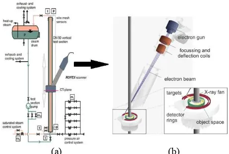
The data analyzed in the present study are carried out from the air-water experiments in DN-50 pipe section at the TOPFLOW facility. An ultrafast X-ray computed-scan tomography is installed at the 54.8 mm diameter titanium vertical pipe with 6 meters tall.The use of titanium pipe is useful for carrying out experiments at high pressure and temperature, also reducing the possible radiation attenuation due to X-ray source. The available length for measurement is about 3.3 m and distributed in 6 dimensionless axial stations (x/D), such as: 0.3 (A), 1.13 (D), 3.12 (G), 7.94 (J), 23.3 (M), 59.7 (P) pipe diameters. A schematic layout of the experimental setup is depicted in Fig. 1 (a).

(a) (b)

Fig. 1. (a) Schematic diagram of DN-50 vertical pipe test (b) Working principle of ROFEX

The experimental condition for slug flow involves the gas-superficial velocity and liquid-superficial velocity ranging from 0.219 to 0.534 m/s and 0.045 to 1.017 m/s, shown in Table 1 and followed by the explanation of used method.

Table 1. Experiments condition Matrix point JG (m/s) JL (m/s) Method

111 0.219 0.0405 Time-series 114 0.219 0.161 Bubble pair 116 0.219 0.405 Time-series 118 0.219 1.017 Bubble pair 133 0.534 0.0405 Time-series 140 0.534 1.017 Bubble pair

B. Working Principle of An Ultrafast X-Ray Tomography

Generally, X-Ray CT-scans work by utilizing the attenuation of radiation which passes through an object. Afterwards, the intensity change of radiation attenuation is recorded by the detectors. However, a high measurement frequency is required for measuring air-water flowdue to their complex interactions and interfacial boundaries.

An ultrafast X-ray tomography namely “ROFEX” (RossendorfFast Electron beam X-ray tomography) is mounted at the DN-50vertical test section of the TOPFLOW experiment facility. The deviceworks by implicating the scanned electron beam principle [22].An electron beam is focused on a circular tungsten target. At the same time, the deflection coils periodically deflect the beam in x-y direction with a high frequency and yield a rotating X-ray fan. This mechanism enables to describe cross-sectional pipe area with very high frequency. A schematic view of the ultrafast X-ray tomography ROFEX is depicted in Fig.1 (b) above. As the non-intrusive device, performance comparison with previous wire-mesh sensor [23] and basic explanations on ROFEX working principle have been explainedby [24, 25].

C. Reconstruction and Segmentation of Tomography Stacks

Results from tomography scanning are stored in the form of matrices, called as “sinogram”. The matrices contains cross-sectional image stacks, defined by the detector number in the horizontal direction and the projection angle in the vertical direction. The data are then processed by means of

filtered back projection algorithm[26].The 3D arrays with specific image gray valuesare scaled up to represent gas and liquid phase distribution based on the pixel ratio. Array dimensionsare 108 x 108 pixels and the array length is depended on selected frequency and measurement time.

To reveal bubble parameters, the gray value arrays should be binarized to obtain interfacial boundaries among gas and liquid. A new algorithm for better segmentation resultwas successfully developed. This algorithm works by tracing maximum local gray values as the beginning of bubble regions and looking the agglomeration possibilities with the surrounding connected pixels[27].This step is repeated until no more connectivity and results bubble regions which are larger than “real bubble”. An individual threshold is used based on maximum bubble gray value (started from 95%). Flow chart of the segmentation process is shown in Fig. 2.

Fig. 2. Flow chart of a new segmentation algorithm [27]

Segmentation derives important bubble parameters including numbers, sizes, detected position in space and time, gas-fraction in whole measurement, and maximum occupied radius in cross-sectional area (rxymax).

D. Bubble Pair Algorithm

In order to obtain more accurate results of bubble velocities and bubble properties as well, an individual recognition based on the highest bubble probabilities is obtained, called as bubble pair algorithm [28, 29]. By looking for similar bubbles which is detected in both measurement planes, each bubble moving position and traveling time can be obtained. Moreover, when two bubbles reach the highest similarities in volume, position, and expected velocity, they are decided as the most suitable paired bubble. A particular method to find each bubble pair probabilities is created. In order to optimize bubble pair method, bubble pair searching is started from largest to smallest size bubbles becausenumbers of large size bubblesless than small size bubbles.

1. Velocity probability

1.1. Calculation of expected velocity

Rise velocity of a bubble in flowing liquids is a superposition of its terminal velocity and the component due to liquid flows. For bubbly flow case, it follows the

power-law distribution equation[30].A modification of [30] with the use of terminal velocity equation by[31] is obtained for expected velocity of bubbly flow case, written in (2):

= 1.2 + (1− )1/6_{+ 0.53} ∆

0.25 ₍₂₎

For the special case of slug flow, the Taylor bubble and bubbles in other different regions were given specific codes in both measurement layers. To simplify the calculation, there are only bubbles with same codes in upper and lower layers areprocessed. Detail explanations of each bubble region are summarized as follow:

a) Taylor bubble (code: 1)

The recognition criteria for Taylor bubble are when 2 (rxy max) > 35 mm and dequiv> 40 mm. Calculation of Uexpis defined by using (3), as revealed by [5]:

Uexp = 1.2( + ) + 0.35 gD (3)

b) Bubble in Falling Film Region (code: 2)

The algorithm also considered the presence of bubbles in falling film region. Expected velocity is obtained from mass-continuity relation by involving falling film velocity

[32],expressed as follow,

Uexp= ( + ) + −( − ) (4)

When Ifront-TBImIback-TBandr 0.5 (rxy max-TB)

c) Extension of Falling Film Region (code: 3)

Falling film region extends until 1 pipe diameter [33] and

creates “swelling” motion inside[32, 33]. Bubbles in this region using the specified criteria: Iback-TBImIback-TB +

(1D/Uexp-TB) and rrxymax-TB. A similar calculation method with

the case of falling film, as in (5) was used to obtain Uexp. Uexp = Uexp-Falling film region (2) (5)

d) Wake region (code: 4)

Wake region extends until around 2 pipe diameter behind the Taylor bubble[34].Therefore, bubbles in wake region were defined if Iback-TBImIbackTB + (2D/Uexp-TB)and do not

assigned as bubbles in falling film. Calculation of Uexp

follows the default expected velocity for bubbly flow case.

e) Bubbly flow region (code: 5)

When a region of liquid slug does not affected by Taylor bubble and wake motion, this region is defined as developed bubble [34],with similar behavior as bubbly flow. Hence, the similar criteria of default bubble pair method were used.

1.2. Calculation of velocity probability

After expected velocity were defined, the difference among the calculated axial velocity and expected velocity

is first determined, called as bubble pair

velocity( ). The velocity range is then calculated by criteria of 0.375 Uexp and the drift velocity. Determination

Table 2. Criteria for velocity range in velocity probability calculation

Table 3Determination of velocity probability Criteria Velocity probability (∅ ) by considering the most identical volume between bubble pair candidates. As a calculation method, Gaussian distribution is used. The equation involves volume difference and sigma parameter which can be represented in (11).

∅ = −0.5 ∆ 2

(11)

The bubble volume is used in this calculation is termed as equivalent volume ( ), as a multiplication of virtual volume, symbolized as (mm2.ms) and one-third power of bubble velocity. This can be written as:

= _� 1/3 (12)

Therefore,

∆ = | (∆ ) −(∆ ) | (13) For the calculation of , the criteria is set to give a range tolerance, stated in Table 4.

Table 4. Criteria for sigma volume in Gaussian function Criteria _{Sigma volume ( )}

zero volume probability (∅ = 0).

3. Position probability

A similar statistical method (Gaussian function) is also implemented to find position probability.

∅ = −0.5 relationship is previewed as in (18),

= 2.5

�

(18)

After all probabilities are calculated, the total probability is determined by multiplication of three probability types. The velocity and volume probabilities consider the bubble movement from lower-upper or upper-lower planes. Thus, total probabilities are determined as follow:

∅ = ∅ _{( )}.∅ _{( )}.∅ _{( )}.∅ _{( )}.∅ ₍₁₉₎

To minimize the bubble selection errors, a simple threshold base on empirical notes is applied. For bubbles which do not reach minimum total probabilities 30% are neglected, or assumed as measurement errors.

E. Data Analysis

1. Bubble size determination

Through X-ray measurement, size of the bubble can be determined by the term of equivalent (Sauter mean) diameter which can be obtained from (20),

= 2 _� 1/3 (20)

where is bubble virtual radius (mm2ms) which calculated from detected virtual volume. For the equivalent diameter, it should be multiplied with one-third power of bubble velocity.

2. Velocity determination

The instantaneous bubble velocity is obtained by bubble displacement (from lower to upper measurement layer) in a particular time. Some criteria are used todetermine time-lag of each bubble displacement, based on the maximum radius of cross sectional area (rxymax). These criteria are

summarized in Table 5.

Table 5. Criteria for time determination Bubble size Time used

rxymax<3 mm Time in center of mass (Im) 3 mm <rxymax<10 mm Interpolation virtual time (Ivir)

rxymax>10 mm Time in front region (Ifront)

Virtual time comes an interpolation calculation between Ifront and Im. Therefore, the three dimensional velocities

can be determined by using bubble pair result and segmentation file database.

a) Three-Dimensional(3D) velocity

Bubble three-dimensional velocity is a composition of both movements in axial and horizontal directions. As a vector, it can be mathematically described as in (21).

฀3 = � 2+ 2 ₍₂₁₎

 Axial velocity ( _� )

Bubble movement in axial distance is derived from the division of gap between measurement planes (10.2 mm) to the time differences, as well described in (22).

� =

10.2

(∆ ) _→ (22)

 Horizontal velocity ( )

During the rising movement, bubble also possible to move laterally along the horizontal direction.Hence, a horizontal velocity is calculated based on the coordinate difference in x(j) and y(k) directions. Velocity calculation is shown as in (23).

=(∆ ) (∆ ) _→ =

( − )2_{+ ( − )}2

(∆) _→ (23)

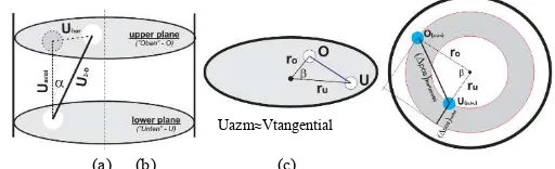
 Polar angle ()

An angle between bubble axial and horizontal movements is defined as a polar angle. According to the trigonometry function, the polar angle is defined as follow:

= −1

� (24)

b) Radial velocity

The bubble lateral movement influences by lift force, whichhas either direction to pipe core region or wall region. Radial velocity considers the bubble movement from inter-cross sectional radius area. Hence, bubble tendency to move can also be determined. In calculation, the radial position difference and the travel time between lower to upper measurement planes are considered, as in (25).

=− (∆ )

(∆ ) _→ =−

−

(∆ ) _→

(25)

wherethe bubble radial position is calculated by (26).

= ( − )2_{+ ( − )}2 (26)

For the radial velocity, negative sign is used to define the bubble tendency. Thus, positive value of radial velocity means bubble tends to move toward pipe center region and vice versa.

c) Azimuthal velocity

A simple analogy of tangential velocity was used to determine azimuthal velocity.

( _� ) _→ =

(∆ ) _→

(27)

where is a symbol for movement direction {-1,0,1} by obtaining the lowest angle possibility between two-radial distances and is an azimuthal angle () which is obtained from (28):

= −1 ∙

= −1

+

2

+ 2 2+ 2

(28)

It should be noted that in this present calculation, the counter-clockwise movement is initialized by positive

sign.For the sake of clarity, illustration of the explained velocities are depicted in Fig.3 below.

(a) (b) (c)

Fig. 3. (a) Preview of bubble three-dimensional rising movement; (b) Bubble azimuthal movement; (c) Bubble horizontal and radial velocities.

3. Taylor bubble and liquid slug length

The individual Taylor bubble length can be determined by the multiplication of Taylor bubble axial velocity and the time difference in each measurement layer. By an assumption of constant bubble nose and tail velocity, liquid slug length behind a Taylor bubble is also determined by the same procedure using velocity of leading Taylor bubble. The procedure is also used to prevent high possibilities of artificial coalescence in bubble tail area [35].

Taylor bubble length is defined as:

= _� ( - ∆ ) (29)

Liquid slug length is defined as:

= � ( ) +1 −( ) (30)

Using the assumption of,

� _{= (}

� ) −1 (31)

4. Bubble frequency

Bubble frequency is defined as the number of bubbles that counted in whole measurement times. Hence, it is stated as bubble/s unit.

5. Averaged cross-sectional void fraction

Time-series data shows the cross-sectional averaged void fraction. Measurements are capable to produce time-series data from upper and lower planes in the form of void fraction signal in time domain.

III.RESULTS AND DISCUSSION

A. General characteristics of co-current upward slug flow Results of averaged cross-sectional void fraction measurement in different axial position show the flow evolution from bubbly to slug flow. Fig.4 (a). shows the transformation from wall-peaking to core-peaking bubble. In the lowest measurement station, bubbles still tend to occupy around the pipe wall. As the increase of axial measurement stations, bubbles agglomerate into the center pipe area, generate larger and elongated bubbles, called as Taylor bubble.Because of the lower turbulence dissipation rate and lower shear rate at the center of the pipe, the bubble can grow into larger bubbles by coalescence with less possibility of breakups [14, 36].

Fig. 4. (a) Averaged time series data for void fraction (114); (b) Effect of liquid superficial velocities on constant gas-superficial velocity to the

average void fraction; (c) Double-peaked curve of slug flow (114-P)

Slug flow pattern is also characterized by the presence of bimodal (double-peak) shape of PDF-graph[37,38], shown in Fig 4 (b). Slug flow is characterized by the presence of gas-slugs(Taylor bubble), dominantly occupied in time-series data of average void fraction. This graph never reach the absolute value of 1.00 due to the existence of small dispersed bubble behind Taylor bubble tail. Average void fraction along the measurement station changes from inlet to exit position, as can be seen in fig. 4 (b). In constant JG of 0.219

m/s, largest void fraction is occupied by matrix point 111 which has lowest JL. It is caused by high gas dominancy

among flow proportion.

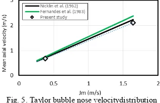
B. Taylor bubble velocity and nose movement

Axial velocity of Taylor bubble is obtained by the superposition of liquid velocity and drift velocity due to buoyancy forces. Fig. 5 shows the averaged velocity for two matrix points 114 and 140.

Fig. 5. Taylor bubble nose velocitydistribution

The average axial velocity follows the equations [5,12], but little bit under-predicted. As the mixture velocity increase, the axial Taylor bubble velocity is also increased. Comparison for each Taylor bubble velocity to the theoretical models [5, 12] is depicted in Fig. 6. The figure also shows that Taylor bubble velocity is distributed between each other.

Fig. 6. Taylor bubble nose velocitydistribution (114-P)

It is important to investigate the reasons of under-predicted results and the distributed velocity.Theoretically, when the high velocity distribution of Taylor bubble still occurs, flow is not developed yet (as fully developed slug). Hence, coalescence and slug formation are still in process[11, 18, 19].

In a fully developed slug flow, the rising velocity of the Taylor bubble can be regarded as steady[39]. The each Taylor bubble velocity difference and under-predicted result might be caused by the less high measurement position (not yet stable slug) and the existence of small dispersed bubbles in the liquid slug separation distances, respectively.

Relationship between Taylor bubble length and axial velocity is presented in Fig. 7, for the data at 114-P. A slight increase of velocity is performed as the increase of Taylor bubble length. Basically, the length increase gives effect to the volume increase which contributes to the drift velocity increase due to buoyancy forces. This condition is agree with experiment by Polonsky et al. [21]for different Taylor bubble lengths.

Fig.7. Relationship between Taylor bubble length to axial velocity (114-P)

The consecutive relations between the leading and the trailing Taylor bubble are also performed in Fig 8. There is a specific relation between Taylor bubble rise velocity and length of liquid slug ahead. Comparing with of the other experimental results [35, 39], it isshowed a good agreement with a good data trend. Commonly, after reach the stable liquid slug length (10-20 D), the trailing and leading Taylor bubbles are in the similar velocity. The present result still shows the fluctuation in 15 D and 23 D because Taylor bubble is still in arrangement as a developing slug. It is also remembered that measurement ofpoint 114, with medium JL

and JG, is conducted in L/D=60 (3.23 m) which has not

generated a fully developed slug yet, whereas the compared data were taken in quite higher measurement position.

(b)

Fig. 8Consecutive relation between Taylor bubbles and their separation distances of liquid slug ahead (114-P)

Taylor bubble nose shapes are found swayed and move side-to-side along the consecutive orders. Fig. 9 (a) illustrates the radial position difference of Taylor bubble nose. Consequently, as the effect of swaying movement, the algorithm detects different nose radial and azimuthal velocities. Fig. 9 (b) illustrates an example of different nose shapes with different radial positions of nose tip. Qualitatively, there are interesting cases in Taylor bubble nose shapes, such as double-noses, double liquid lamellas, and the other shapes, which may depends on the liquid and wave generated by the separation distance ahead. These phenomena become one of the complexity in slug flow.

(a) (b) Fig. 9.(a) Radial distribution of Taylor bubble nose velocity(114-P);

(b) Example of Taylor bubble nose swaying movement

The nose tip is possibly tends to the pipe wall or pipe center, following the maximum velocity profile ahead it. Reason of the swaying movement are also strengthened by Mayor et al. [41],who conducted that the nose follows the fastest portion of fluid ahead, resulted in continuous elongations and relaxations of the bubble shape. Moreover, Taylor bubble shape is varying and the bubble nose sways from one to other sides because most dispersed bubbles in the liquid slug are consumed by the elongated bubbles, but some of them penetrate into the liquid[42]. Coalesce of small bubbles to nose also possible to be a reason of the detected radial velocity change, as the effect of wrong detected time of front Taylor bubble position. The small bubble coalescence to nose mechanism has been explained by [43], as the result of re-coalesces back action due to out-of-controlled wake and vortices in liquid slugs. A different behavior of whole Taylor bubble body and nose tip is showed in the measurement of movement angles, expressed in Fig. 10 (a) for polar angle and

(b) for azimuthal angle. The whole Taylor bubble body polar angle, contributed by axial and horizontal velocities, is relatively small but the discrepancies occur in the nose polar angles. It can be concluded that body and middle area of Taylor bubble always move upward in straight axial direction, but the nose may performs the lateral movements. The nose azimuthal angle also varies. The variation leads the helical mechanism of nose upward movement. If the wave profile ahead the nose is considered, it becomes a possible reason for different nose shapesincluding the double-noses. Once again, this result confirmed the nose sways mechanism occurs, especially in developing slug flow.

(a) (b)

Fig. 10. (a) Measurement of polar angle in whole Taylor bubble body and its nose; (b) Histogram of azimuthal angle of Taylor bubble nose

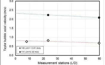
Effect of the measurement stations to the Taylor bubble velocity is previewed in Fig. 11. As the increase of measurement station, Taylor bubble velocity is not quite influenced, but the velocity seems a slightly decrease. This phenomenon is in a good agreement with experiment in 54 mm pipe diameter by Van Houtet al. [11] for the L/D = 16.8 and 50.4. The experiments was conducted by probe and image processing. The translational velocity tend to decrease first in the developing stations and increase at L/D = 88.7 to 127. Measurements in points 140 and 114 show the similar trends, but Taylor bubbles are only formed and detected since measurement station J.

Fig. 11. Effect on measurement stations on Taylor bubble axial velocity

C. Taylor bubble and liquid-slug length

Fig. 12. Effect on measurement stations on the average length of Taylor bubble and liquid slug [matrix point: 114 and 140)

When the trend is compared with result of time-series data, higher measurement station affects longer and wider time durations of high-void fraction peak and the separation distance, shown in Fig. 13.In this diagram, the averaged void fraction signal for matrix point 133 P and M are presented. It is obviously shown that the highest station is consisted of

longer and wider “signal” rather than the lower stations.

Additionally,the matrix point 133 is the lowest liquid superficial velocity which generates much longer Taylor bubble due to the gas-phase dominancy in two-phase flow.

Fig. 13. Example of time-series data in different measurement positions (taken from matrix point 133 P and M)

D. Flow development effects

In the slug flow case, bubble pair algorithm is capable to identified bubbles in differentslug flow regions, based on the previous criteria. As the result, bubble frequency can be calculated. Fig. 14 performs the frequency of solved dispersed bubbles in liquid slug region along 10 seconds measurement time for 114-P matrix data. In this figure, classified wake and swelling (falling film extension) appear since at the D-station. It has a meaning that spherical cap bubbles also generates small wake and falling film effects.

Fig. 14. Effect of measurement stations on thesmall bubbles frequency (114)

Frequency of developed bubble is relatively stable, due to the nature of bubbly flows. When the Taylor bubble begin to appear (J-station), liquid slug is also generated, decreasing the bubbles in wake, falling film, and swelling and increasing the developed bubble frequency. This phenomena occurs because

longer liquid slugs open the chance for bubble to be more dispersed and act like a natural bubbly flow (weaker wake and falling film effects). This argument isan in line agreement with Van Hout et al. [34] who define developed bubble flow is a normalized condition after intermediate condition and wake region (length until 2D).In addition, the frequency decrease is might be caused by the small dispersed bubble coalescence during the growth of Taylor bubbles and liquid slugs. It observed the swelling region has steep decreasing slope than the others. Fig. 15 (a) shows the chaotic mixing region in Taylor bubble rear area[44]. In the region, bubbles in wake, swelling, and falling film regions can meet together and the possibility to coalesce is able to take place. Although the average equivalent diameters for the four kinds of bubbles are relatively constant, Fig. 15(b) presents that the diameter in wake region is always little bit higher in every measurement stations. In the experiment of 26 mm diameter, Zheng et al.

[44] was also stated the higher diameter of bubbles in wake region is presented rather than the small dispersed bubbles.

Fig. 15. (a) Effect on measurement stations on Taylor bubble axial velocity; (b) Entraiment formation in the behind Taylor bubble (taken from [44]).

The presence of large-skirted bubble is usually known as

“spherical cap bubbles”[4, 45], defined as a large bubble with 20 mm dequivDpipe was defined as spherical cap bubble

[8,9].In the Fig. 16 (a), the development of cap bubbles and Taylor bubbles are presented. The larger bubbles grow as Cap bubbles and located into pipe center, because there are lower rate of turbulence dissipation and lower shear rate than in around pipe wall [14, 15].

(a) (b)

Fig. 16. (a) Effect on measurement stations on Taylor bubble and cap bubbles frequency; (b) Preview of Taylor bubble and cap bubble coalescence (114 M)

Since the J-station, Taylor bubble start to grow and caps bubble frequency is decreased because of the coalesce intention to the Taylor bubbles or the other cap bubbles. Fig. 16 (b) displays an example of bubble coalescence in 114-M, where is a developing station. Contrarily, Taylor bubble numbers through J and M stations are increased. The bubble Avera

ged void fractio n (%)

(a)

agglomeration results more bubbles with dequiv>dpipe, which is

recorded by the algorithm as a Taylor bubble. The Taylor bubble is still going to become larger and longer again, as long as the increase of measurement stations. At those points, coalescence may still occurs. Hence, a slight frequency decrease is shown in P-station.

E. Bubbles in liquid slug

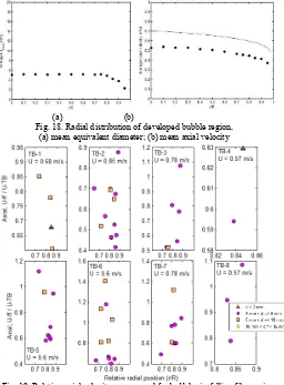
Previously, theindividual characteristics of small dispersed bubble in liquid slug is still rarely characterized. The high dense flows, swarm dispersed bubbles with high shear stress in Taylor bubble rear area, and also the generated vortices by wake region are contributed to the difficulties of the segmentation process. They also become a reason of the visual limitations. Therefore, only the result trends are discussed and compared with the previous results. Fig. 17 (a) and (b) present the distributions of bubble equivalent diameter. These diagrams are only approach method thatshow the diameter trend. In developed bubble region, average diameter is reached around 5-5.5 mm and larger distribution is occurred in wake region. However, bigger diametersare possibly caused by artificial coalescence due to the difficulties to define interface boundaries in very small and chaotic movements of bubbles in wake region. Fig 18 (a) and (b) depict the average equivalent diameter and mean axial velocity, respectively. In near pipe wall, the bubble diameters decrease so that this area is occupied by smaller bubble diameters. The mean axial velocity follows power-law distribution curve [30] which representsthe nature of bubbly flow.

Fig. 17. Distribution of bubble equivalent diameter in (a) developed bubble region and (b) wake region (point 114-P)

Axial velocity of small bubbles in liquid falling film, normalized by each Taylor bubble velocity (8 bubbles in 114-P) are shown in Fig. 19. Most bubbles located in near pipe wall (relative radial positions starting from 0.6 to 0.9) due to swept effect of Taylor bubble rises. The velocity is expected less than Taylor bubble velocity (less than 1). Taylor bubble velocity is faster than its surrounding. Bubble diameter distributions are around 3-6 mm and 6-10 mm in near wall and slightly centered, respectively. However, bubbles with larger velocity are might be an artificial coalescence to the Taylor bubble body or nose which detected has a same or even larger velocity with the Taylor bubble.

(a) (b)

Fig. 18. Radial distribution of developed bubble region, (a) mean equivalent diameter; (b) mean axial velocity

Fig. 19. Relative axial velocity – compared for bubbles in falling film region

V. SUMMARY AND CONCLUSIONS

Determination of Taylor bubble properties from temporal and spatial experimental database of ultrafast X-ray tomography is carried out. Identification of paired bubble from bubble pair methods plays an important role in determination of bubble properties and capable as an approach method to characterize high density flow, such as small dispersed bubble in liquid slugs. Flow development affects the slug flow characteristics and Taylor bubble evolution. It is concluded that distribution of Taylor bubble velocities caused by the condition of developing slug flow and the presence of small bubbles in the liquid slug (in the form of wake influence) which responsible to the nose movement and the drift velocity. Comparison of the previous results strengthened the physical understanding of gas-liquid slug flow.

ACKNOWLEDGMENT

This work is a collaboration between GadjahMada University-Indonesia and HZDR-Germany. Akmal Irfan Majid acknowledges support from Institute of Fluid Dynamics of HZDR during 4-months stay at HZDR and grantee of Fast-Track Master Program Scholarship from Ministry of Education and Culture of Republic of Indonesia.

The present work was carried out in the frame of research project funded by German Federal Ministry of Economics Affair and Energy, project number 150 1411.

REFERENCES

[1] Taitel, Y., Barnea, D., Dukler, A.E., “Modeling Flow Pattern Transition for Steady Upward Gas-Liquid Flow in Vertical Tubes”, American Institute of Chemical Engineering Journal, 26, pp. 345-354, 1980. [2] Hewitt, G.F., Hall-Taylor, N.S., Annular Two-Phase Flow, Pergamon

Press, 1970.

[3] Dumitrescu, D.T.Z., “Strömung an EinerLuftblaseimSenkrechten Rohr”, Z. angew. Math. Mech., 23, 139, 1943.

[4] Taylor G.S., Davies, R.M., “The mechanics of large bubbles rising through extended liquids and through liquids and through liquids in tube, Proc. R. Soc. London, Ser. A, 200, 375, 1950.

[5] Nicklin, D.J., Wilkes, J.O., and Davidson, J.F., 1962, Two-Phase Flow in Vertical Tubes, Trans. Inst. Chem. Engrs, 40, 61.

[6] Zukoski, E.E., “Influence of viscosity, surface tension, and inclination

angle on motion of long bubbles in closed tubes,” J. Fluid Mech., 25, 821, 1966.

[7] Tomiyama, A., Nakahara, Y., Adachi, Y., Hosokawa, S., “Shapes and

rising velocities of single bubbles rising through an inner subchannel,”

J. Nucl. Sci. Technol., 40, 136, 2003.

[8] Krüssenberg, A.-K., Prasser, H.-M., Schaffrath, A., “A new criterion for

the bubble slug transition in vertical tubes”, Proceeding of 9th International Topical Meeting on Nuclear Reactor Thermal Hydraulics (NURETH-9), San Francisco CA, 3–8 October, 1999.

[9] Lucas, D., Krepper, E., Prasser, H.-M, “Development of co-current air–

water flow in a vertical pipe”, International Journal of Multiphase Flow, 31, pp. 1304–1328, 2005.

[10] Prasser, H.-M., Scholz, D., Zippe, C., “Bubble size measurement using wire-mesh sensors”, Flow Measure. Instrument., 12, pp. 299–312, 2001. [11] Van Hout, R., Barnea, D., Shemer, L., “Translational velocities of

elongated bubbles in continuous slug flow”, Int. J. Multiphase Flow, 28, pp. 1333-1350, 2002.

[12] Fernandes, R.C., Semiat, R., Dukler, A.E., “Hydrodynamic Model for Gas-Liquid Slug Flow in Vertical Tubes”, American Institute of Chemical Engineering Journal, 29, pp. 981-989, 1983.

[13] White, E.T., Beardmore, R.H., “The velocity of rise single cylindrical

air bubbles through liquid contained in vertical tubes”, Chemical Engineering Sciences, 17, pp. 351-361, 1962.

[14] Lucas, D., Krepper, E., “CFD Models for Polydispersed Bubbly Flow”,

HZDR Technical Report FZD-486, HZDR-Germany, 2007.

[15] Krepper, E., Lucas, D., Frank, T., Prasser, H.-M., Zwart, P.J., “The inhomogeneous MUSIG model for the simulation of polydispersed

flow”, Nuclear Engineering and Design, 238, pp. 1690–1702, 2008 [16] Van Hout, R., Barnea, D., Shemer, L., 2001, “Evolution of statistical

parameters of gas-liquid slug flow along vertical pipes”, International Journal of Multiphase Flow, 27, pp. 1579-1602, 2001.

[17] Mao, Z.S., Dukler, A.E., “An experimental study of gas-liquid slug

flow”, Experiments in Fluids, 8, pp. 169-182, 1989.

[18] Pinto, AMFR, Campos, JBLM, “Coalescence of two gas slugs rising in

a vertical column of liquid”, Chemical Engineering Science, Vol. 51, 1, pp. 45-54, 1996.

[19] Pinto, A.M.F.R., Coelho Pinheiro, M.N., Campos, J.B.L.M.,

“Coalescence of two gas slugs rising in a co-current flowing liquid in

vertical tubes”, ChemEngSci, 53, pp. 2973–2983.

[20] Shemer, L., Barnea, D., “Visualization of the instantaneous velocity profiles in gas–liquid slug flow”, Physic. Chem. Hydrodyn., vol. 8, pp. 243–253, 1987.

[21] Polonsky, S., Barnea, D., Shemer, L., “Averaged and time dependent characteristics of the motion of an elongated bubble in

a vertical pipe”, Int. J. Multiphase Flow, vol. 25, pp. 795–812, 1999a. [22] Hampel, U., et al., “Experimental ultrafast X-ray computed tomography

with a linearly scanned electron beam source”, Flow Measurement and Instrumentation, 16, pp. 65–72, 2005.

[23] Prasser, H.-M., Misawa, M., Tiseanu, I., “Comparison between wire -mesh sensor and ultra-fast X-ray tomograph for an air–water flow in a

vertical pipe”. Flow Measure. Instrument. 16, 73–83, 2005.

[24] Fischer, F., et al., “An Ultrafast Electron Beam X-ray Tomography Scanner”, Measurement in Science and Technology, 19, 2008.

[25] Fischer, F., Hampel, U., “Ultrafast Electron Beam X-ray Computerd Tomography for Two-Phase Flow Measurement”, Nuclear Engineering and Design, 240, pp. 2254-2259, 2010.

[26] Kak, A. C. and Slaney, M., Principles of computerized tomographic imaging, IEEE Press, 1988.

[27] Banowski, M., Lucas, D., Hoppe, D., Beyer, M., Szalinski, L., Hampel,

U., “Segmentation of ultrafast x-ray tomographed gas-liquid flows in a vertical pipe at different flow regimes”, Proceeding of 7th _World

Congress on Industrial Process Tomography, Krakow-Poland, 2013. [28] Patmonoaji, A. “Investigation of gas-bubble velocities from

experimental data of ultrafast two-layer electron beam X-ray

tomography”, Master Thesis, GadjahMada University, Indonesia, 2014. [29] Patmonoaji, A., Banowski, M., Lucas, D., Deendarlianto, “Investigation

of gas-bubble velocities from experimental data of ultrafast two-layer electron beam X-ray tomography”, Proceeding of The 12th _Annual

National Seminar of Mechanical Engineering (SNTTMXII), Bandar Lampung-Indonesia, pp. 1374-1383, 2013.

[30] Bankoff, S. G., “A variable density single-fluid model for two-phase flow with particular reference to steam-water flow”, J. Heat Transfer, 82 (2), pp. 265-270, 1960.

[31] Harmathy, T.Z., “Velocity of Large Drops and Bubbles in Media of

Infinite or Restricted Extent”, American Institute of Chemical Engineering Journal, 6, 281, 1960.

[32] Ahmad, W.R., DeJesus, J.M., Kawaji, M., “Falling film hydrodynamics in slug flow”, Chem. Eng. Sci, 53, pp. 123-130, 1998.

[33] Kawaji, M., DeJesus, J.M., Tudose, G., “Investigation of flow structures

in vertical slug flow”, Nuclear Engineering and Design, 175, pp. 37-48, 1997.

[34] Van Hout, R., Shemer, L., Barnea, D., “Spatial distribution of void fraction within a liquid slug and some other related slug-parameter”, Int. J. Multiphase Flow, 18, pp. 831-845, 1992.

[35] Guo-dong, X., Zhen-zhen, C., Qing, L., “A model for liquid slug length distribution in vertical gas-liquid slug flow”, Journal of Hydrodynamics, 21 (4), pp. 491-498, 2009.

[36] Kaji, R., Azzopardi, B.J., Lucas, D., “Investigation of flow development of co-current gas–liquid vertical slug flow”, International Journal of Multiphase Flow, 35, pp. 335–348, 2009.

[37] Costigan, G., Whalley, P.B., “Slug flow regime identification from dynamic void fraction measurements in vertical air–water flows”, Int. J. Multiphase Flow, 23, pp. 228–263, 1996.

[38] Khatib, Z., Richardson, J.F., “Vertical co-current flow of air and shear thinning suspensions of kaolin”, Chem. Eng. Res. Design, 62, pp. 139-154, 1984.

[39] Moissis, R., Griffith, P., “Entrance effects in a two-phase slug flow”, J. Heat Transfer, 84, pp. 29-39, 1962.

[40] Polonsky, S., Shemer, L., Barnea, D., “The relation between the Taylor bubble motion and the velocity field ahead of it”, International Journal of Multiphase Flow, 25, pp. 957-975, 1999b.

[41] Mayor, T.S., Ferreira, V., Pinto, A.M.F.R., Campos, J.B.L.M.,

“Hydrodynamics of gas–liquid slug flow along vertical pipes in turbulent regime –An experimental study”, Int. J. Heat Fluid Flow, 29, pp. 1039-1053, 2008.

[42] Shemer, L., “Hydrodynamic and statistical parameters of slug flow”,

International Journal of Heat and Fluid Flow 24, pp. 334–344, 2003. [43] Yan, K., Che, D., “Hydrodynamic and mass transfer characteristics of

slug flow in a vertical pipe with and without dispersed small bubbles”,

International Journal of Multiphase Flow, 37, pp. 299–325, 2011. [44] Zheng, D., Che, D., “Experimental study on hydrodynamic

characteristics of upward gas–liquid slug flow”, International Journal of Multiphase Flow, 32, pp. 1191–1218, 2006

[45] Joseph, D. “Rise velocity of a spherical cap bubble”, J. Fluid Mech.,