On detectable and non-detectable structural
change
David F. Hendry *
Nuffield College,New Road,Oxford OX1 1NF, UK
Abstract
A range of parameter changes in I(1) cointegrated time series are not reflected in econometric models thereof, in that many shifts are not easily detected by conventional tests. The breaks in question are changes that leave the unconditional expectations of the I(0) components unaltered. Thus, dynamics, adjustment speeds etc. may alter without detection. However, shifts in long-run means are generally noticeable. Using the VECM model class, the paper discusses such results, explains why they occur, and uses Monte Carlo experiments to illustrate the contrasting ease of detection of ‘deterministic’ and ‘stochastic’ shifts. © 2000 Elsevier Science B.V. All rights reserved.
JEL classification:C15; C53
Keywords:Cointegrated time series; Parameter changes; Forecast error
www.elsevier.nl/locate/strueco
1. Introduction
Structural change and dynamics are inherent facets of economic life, and over recorded history have revolutionized the human condition: statistical tests are not needed to discriminate between conditions in 1899 and 1999. Nevertheless, it transpires that a range of parameter changes in econometric models cannot be easily detected by conventional tests, whereas other changes are manifest and easy to detect. The former class includes changes that leave unaltered the unconditional expectations of non-integrated (denotedI(0)) components even if dynamics, adjust-ment speeds, and intercepts are radically altered. The later class comprises shifts in those unconditional expectations. Some related illustrations are provided in Hendry and Doornik (1997), Clements and Hendry (1998).
This paper extends those studies, using a co-integrated vector autoregression (CVAR) as the general model. The analytical framework is the taxonomy of possible sources of forecast error developed in Clements and Hendry (1994), which highlights the impact of various forms of structural break in closed dynamic systems, and allows some surprising predictions about which parameters of a VAR can be altered without much impact on the properties of the resulting data. In matching Monte Carlo experiments, a bivariate system is subject to two structural breaks in its parameters, where the second re-instates the original parameter values, to show the contrast between the ‘detectable’ and (relatively) ‘non-detectable’ changes.1
For example, even when the general data are integrated of order unity (I(1)), the intercepts and the dynamic coefficients of a CVAR can be changed considerably (i.e. by more than 50%), yet parameter-constancy tests do not detect such changes. Moreover, this is not due to model mis-specification: the in-sample model considered here coincides with the data generation process (DGP). Nor is it a matter of generically low-powered tests: the same tests have high power to detect other shifts in either intercepts or dynamic coefficients. The paper explains why this outcome occurs: for more general studies of the size and power properties of parameter-constancy tests in bothI(0) andI(1) systems, see Anderson et al. (1993), Hylleberg et al. (1993).
To summarize why non-detectability occurs, letytdenote a vectorI(0) time series with actual unconditional expectations and variances denoted by E[yt] and V[yt] respectively. Let the corresponding expectations, based on assuming the model is the in-sample DGP, be denoted byE[yt] and V[yt] (an alternative notation might
beEM[·]). Then so long asV[yt] is not markedly different from V[yt], detectability
depends strongly on the differenceE[yt]−E[yt]. Consequently, parameter changes
in the class that leaveE[yt]#E[yt], suffer from a detectability problem unless they
generate large variance increases. Since I(1) CVARs can be reparameterized by differencing and cointegration transformations asI(0) vector equilibrium-correction models (VEqCMs), where all variables are expressed as deviations around their (pre-break) means, the same logic applies: only shifts in those means induce departures that are readily detectable. Indeed, it is easy to create major parameter shifts that leave the first two moments virtually unchanged, and such breaks will be almost impossible to detect using tests based on those moments. Although other aspects of the model might reveal such shifts, including residual auto-correlation when dynamics alter, the correct interpretation would not be obvious, and indeed other tests could well be distorted by the mis-specification deriving from the break. Different tests might be developed to prise out the correct underlying state of nature, but here we focus on the properties of recursively-computed F-tests of parameter constancy, and the associated recursive parameter estimates.
The structure of the paper is as follows. Section 2 describes then-dimensionalI(1) DGP that forms the class within which the analysis is undertaken. Section 3
formalizes the structural breaks to be studied, and Section 3.1 discusses which changes are and are not easily detected. This is followed by a Monte Carlo study of a bivariateI(1) CVAR in Section 4, for three classes of structural break, and in Section 4.5 for shifts in the cointegration space. Section 5 offers potential explana-tions for the mixture of results obtained and Section 6 concludes.
2. The data generation process
Consider a first-order vector autoregression in n variables denoted xt:
xt=t+Gxt−1+nt (1)
where ntINn(0,Vn) denotes an independent, normal error with expectation
E[nt]=0 and variance matrix V[nt]=Vn. The data are assumed to be integrated of order unity (I(1)), perhaps after suitable transformations (such as logs), represented by:
G=In+ab% (2)
whereaandbaren×rmatrices of rankr. All eigenvalues ofGlie on or inside the unit circle, to exclude explosive processes, and to excludeI(2), rank (a%ÞGbÞ)=(n−
r), where aÞ and bÞare n×(n−r) matrices of rank (n−r) and a%aÞ=b%bÞ=0 (although the analysis could be generalized to accommodateI(2) data). Additional lags are easily added, but do not seem to materially affect the outcomes, although linearity may do (primarily because most non-linear functions entail nonzero means, an issue of importance below). The parameters will be allowed to shift, which induces structural change in the system.
In (1):
t=g−am (3)
where m is r×1, and to ensure the appropriate number of ‘free’ parameters,
b%g=0. Substituting Eqns. (2) and (3) into (1) yields the vector equilibrium-correc-tion model (denoted VEqCM):
Dxt−g=a(b%xt−1−m)+nt (4)
where Dxt and bxt are I(0). From Eq. (4), E[Dxt]=g (the unconditional growth rate) soE[b%xt]=m defines the equilibrium means.
2.1.Parameter-constancy tests
3. Structural change
Under structural change, any or all ofg,a,b,morVn, could alter (or indeed the forms of the relationships in the system, the distributional assumptions, and lag lengths, but these are not considered here). Situations such as economic transition undoubtedly involve changes to cointegration links and growth rates, as well as to speeds of adjustment and equilibrium means. We will focus on the more ‘normal’ setting where g, a, or m shift. However, changes that involve setting a=0, or changinga=0to a non-zero value, inherently involve changes in the cointegration structure, and these are investigated below. Changes tobcould be studied, but pose rather different problems, as discussed later. Finally, changes toVnare predicted by the following theory to have less of an impact, unless they are very large, so are not considered here.
Individual realizations of integrated time series almost inherently have non-zero data means, by force of their stochastic trends. Nevertheless, the I(0) components could have zero unconditional means, depending on the form of data transforma-tion and units of measurement. Thus, in order to clarify the impacts of parameter changes, we also write the system Eq. (4) inI(0) space for thenvariablesyt, the first
rof which are theb%xtand the remainingn−rare the relevant elements ofDxt(e.g.
Dxt which ensures a non-singular representation). Of course, this representation is inappropriate whenb can alter. Thus:
yt=f+Pyt−1+et with etINn(0,Ve). (5)
The unconditional expectation (or long-run mean)E[yt] ofytover t=1,…,T is:
E[yt]=(I−P)−1
f=8 (6)
since the earlier assumptions ensure thatPhas all its eigenvalues less than unity in absolute value, leading to the homogeneous specification:
yt−8=P(yt−1−8)+ot. (7)
Under the assumption of constant parameters, Eq. (7) would deliver the one-step ahead outcome (assuming known parameters):
yT+1−8=P(yT−8)+oT+1. (8)
At time periodT, however, we let (f:P) change to (f*:P*), so fromT+1 onwards, the data are generated by:
yT+h=f*+P*yT+h−1+oT+h, h]1.
We assumeP* still has all its eigenvalues less than unity in absolute value, and that the number and form of the cointegrating vectors remains the same. Let
8*=(In−P*)−1
f*, then:
yT+h−8*=P*(yT+h−1−8*)+oT+h. (9)
when 8 is unchanged, so we consider that issue first. We refer to shifts in 8 as ‘deterministic’ changes (since they change the long-run mean), whereas shifts inf
andP that leave8 unchanged are referred to as ‘stochastic’ or ‘non-deterministic’, even though they might involve a changed intercept.
Let oT+1/Tdenote the difference between Eqs. (8) and (9) at one-step ahead:
oT+1/T=8*+P*(yT−8*)+oT+1−(8+P(yT−8)+oT+1)
=8*−8+P*(yT−8*)−P(yT−8) =(In−P*)(8*−8)+(P*−P)(yT−8)
(10)
This would be the expected one-step ahead forecast error from using Eq. (8) as a model when Eq. (9) is the DGP, and all parameters are known. The first term on the last line is the equilibrium-mean shift, and the second is the slope change, which has an unconditional expectation of zero. Indeed, if a slope change occurred when the economy was near equilibrium, soyT#8 and8did not alter, thenoT+1/T#0. Of course, if the economy was in substantial disequilibrium, a larger effect would result, but this seems to part of the explanation for the non-detectability of shifts in f andP that leave 8 unchanged.
3.1.Detectable shifts
We now show that deterministic shifts, namely shifts from 8 to 8*, whether induced by changes in the interceptf, or indirectly by changes in dynamics (i.e. via (In−P*)−1
f) are a detectable failure in linear dynamic econometric systems. We then demonstrate that even if every parameter alters, but this leaves the ‘long-run means’ 8 unchanged, so f*=(In−P*)8, structural change is not easily detected. Indeed, shifts in f, P with constant 8 transpire to be isomorphic to changes in mean-zero processes, wheref=f*=0. Further, while breaks inPalone can cause forecast failures, their ease of detection depends on the magnitudes of the long-run means of theI(0) components relative to their error standard deviations. As Hendry and Doornik (1997) remark, when the long-run mean is non-zero, breaks shift the location of the data, inducing a short-run ‘trend’ to the new equilibrium mean, which is more easily detected than a one-off variance change around the origin. If Eq. (4) had additional dynamics, these could be expressed in growth-rate form, and hence re-written to have zero means around (the equivalent of) g, so the same argument about detectability would apply to shifts in their parameters.
Because the system is dynamic, the impact of any break takes time to have its full effect, and for the system to reach a new equilibrium, so the data expectations alter in every period, making the process highly non-stationary. To develop the primary implications, we just consider the first period following a change, denoted timeT: later periods are amenable to analysis, as are successive changes, although the algebra becomes increasingly complicated. Let denote an estimate, so the forecast
oˆT+1/T=f*+P*yT+oT+1−f. −P. yT (11)
We treat finite-sample biases in estimators as negligible (see Hendry, 1997, for an explanation), so set E[P. ]=P and E[f.]=f. Further, as almost all estimation methods match data means in-sample,8ˆ=(In−P. )−1
f.. LetEdenote the expected value computed from the model, namely, the actual mean of the forecasts given the in-sample parameter values, when Eq. (5) is assumed to hold (i.e. in ignorance of the shift), then conditional onyT:
E[yˆT+1/TyT]=f+PyT.
This is to be contrasted with the actual data expectation at T+1:
E[yˆT+1/TyT]=f*+P*yT.
Then, detectability depends primarily onE[yT+1yT]−E[yˆT+1/TyT]. More precisely from Eq. (11):
E[oˆT+1/TyT]=f*+P*yT+E[oT+1]−E[f. ]−E[P. ]yT
E[oˆT+1/TyT]=f*−f+(P*−P)yT
E[oˆT+1/TyT]=E[yT+1/TyT]= −E[yˆT+1/T/yT].
(12)
Moreover, taking the unconditional means of each term using Eq. (6):
E[yˆT+1/T]=f+PE[yT]=(In−P)8+P8=8 (13)
This is simply the first term in the last line of Eq. (10)
The key implication from Eq. (14) is thatE[yT+1]=E[yˆT+1/T] when8*=8. This
can occur despite changes in the dynamics, represented by shifts inP, or changes inf: for example, if {yt} is a mean-zero process; if8does not change; or if shifts inf* offset those inP* to leave 8constant, despite both dynamics and intercepts shifting. Further, for a given value of (8*−8), the ellect is larger or smaller as
(In−P*) moves closer to (further from) zero.
Of course, the detectability of any shifts depends on their magnitude relative to the error standard deviations. LetVo
whereKfC,ot+
=KotINn[0,In] and C=KPK
−1 (since
C and P are related by a similarity transform, the ordering-dependence of the transformation by K does not matter here). Then, after the break:
E[yT+1+ ]−E[yˆT+1/T+ ]=K(In−P*)(8*−8).
This is the appropriate metric for judging the ‘magnitude’ of a break.
We now illustrate the implications of this analysis for detecting structural change, using some numerical simulations of parameter-constancy tests. Although the above analysis only applies to one-step ahead errors after a single break, the Monte Carlo will examine many forecast (break-test) horizons, and allows for two shifts. Nevertheless, the implications will be seen to hold more generally.
4. AnI(1) Monte Carlo
The Monte Carlo simulation considers the following experiments, implemented in Ox by PcNaive for Windows (see Doornik, 1996; Doornik and Hendry, 1998). The data are generated by a bivariate cointegratedI(1) VAR:
Dx1,t=g1+a1(x1,t−1−x2,t−1−m1)+o1,t
Dx2,t=g2+a2(x1,t−1−x2,t−1−m1)+o2,t
(15)
where oi,tIN[0,sii], with E[o1,to2,s]=0 Öt,s, so in Eq. (15), K is diagonal with elements,sii. We consider four types of experiment:
1. a constant DGP (to establish actual test size)
2. breaks in the coefficients of the feedbacks (a1 and a2) 3. breaks in the long-run mean (m1)
4. breaks in the growth rates (g1 and g2).
Four different full-sample sizes are considered T=24, 60, 100, and 200 (de-noted a, b, c, d on graphs), the last of which is relatively large for macro-eco-nomic models. Breaks occur at t=0.5T, and revert to the original parameter values at t=0.75T to mimic a second break. Thus, the design seeks to isolate the effects of more information at larger T with fixed relative break points: as will be seen, ‘undetectable’ breaks remain hard to find even at the largest sample size considered here. Since breaks are involved, these experiments could not have been conducted as one recursive experiment from T=10 to 200, except when studying null rejection frequencies. However, for graphical presentation, the indi-vidual graph lines between a, b, c, d are only distinguished by a different symbol where that clarifies an important feature, even when the recorded outcomes overlap.
imposed, but doing so is unlikely to affect the rankings across the outcomes in our experiments 1 – 4. Throughout, 500 replications were used, and rejection fre-quencies at both 0.05 and 0.01 nominal test sizes were recorded (so have stan-dard errors of about 0.01 and 0.004, respectively).
The experimental formulation is invariant to what induces changes in gi−
aim1, but large growth-rate changes seem unlikely in real economic variables. It may seem surprising that the ‘absolute’ size of m1, can matter, since even after log transforms, the measurement units affect m1: for example, a switch from a price index normalized at unity to one normalized at 100 radically alters m1 in (say) a log-linear money-demand model without affecting either a or s. Never-theless, changes in m1 (relative to error standard deviations) also need to be judged absolutely, not as percentages: thus, using 9 to denote parameter changes, 9m1/s matters per se, and this cannot depend on the measurement system, only on agent’s behaviour. When m1/s is large (small), a given effect will be a small (large) percent, but will have the same detectability for a givena. For example, for both broad and narrow money demand in the UK after financial innovation in the mid 1980s (see Hendry and Ericsson, 1991; Ericsson et al., 1998), 9m1/s#25 – 30, in models that excluded appropriate modifiers. The rise in the savings rate in the mid 1970s was of roughly the same absolute magnitude (see e.g. Hendry, 1994). For ‘standard’ values of a, (around 0.1 – 0.2) these num-bers translate into ‘permanent’ equilibrium shifts of 2.5s– 6s. Such consider-ations determined the values of the parameters in the experimental design.
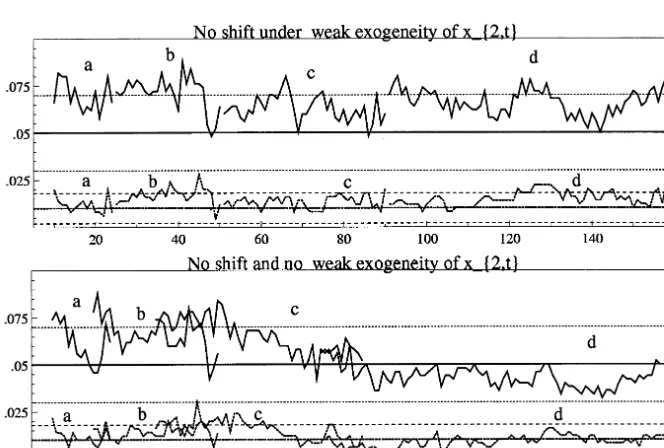
4.1.Test size
The relation of the actual to the nominal size for vector constancy tests has not been much investigated, so the experiments in (1) check their size in an I(1), cointegrated setting, with and without feedback in the second equation. As Fig. 1 reveals, the results are reasonably reassuring when the EqCM enters both relations: with 500 replications, the approximate 95% confidence intervals are (0.03, 0.07) and (0.002, 0.018) for 5% and 1% nominal, and these are shown on the graphs as dotted and dashed lines respectively, revealing that few null rejection frequencies lie outside those bounds once the sample size exceeds 60. At the smallest sample sizes, there is some over-rejection, though never above 9% for the 5% nominal or 3% for the 1% nominal. When the EqCM enters the first relation only, there is a systematic, but small, excess rejection: around 6% instead of 5%, and 1.5% instead of 1%. However, these outcomes are not sufficiently discrepant to markedly affect the outcomes of the ‘power’ comparisons below.
4.2.Dynamic shift
Experiments in (2) demonstrate that a change in the strength of reaction to a zero-mean disequilibrium is not readily detectable. This is despite the fact that the intercept also shifts in the VAR representation:
Fig. 2. Constancy-test rejection frequencies for changes ina. xt=g−am+ab%xt−1+ot pre break
xs=g−a*m+a*b%xs−1+os post break.
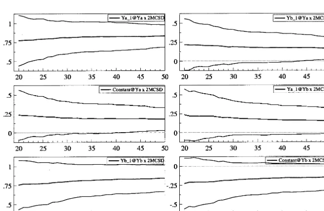
One might have anticipated detectablity from 9am"0, particularly since that change numerically exceeds the equivalent jump in (3) which we show below is easily detected. Nevertheless, despite the induced intercept shift, changes in the dynamics alone are not easily detectable. Fig. 2 records the outcomes: the powers are so low, do not increase with sample size, and indeed barely reflect any breaks, that one might question whether the Monte Carlo was correctly implemented: be assured it was, but anyway, this effect is easy to replicate using PcNaive. Moreover, it was predicted by the analysis above, by that in Clements and Hendry (1994), and has been found in a different setting by Hendry and Doornik (1997), so is not likely to be spurious.Further, the presence of an additional EqCM feedback does not influence these results, even though one might expect an induced shift. Perhaps other tests could detect this type of change, but they will need some other principle of construction than that used here if power is to be noticeably increased. Although direct testing of the parameters seems an obvious approach, as Fig. 3 shows, there is no evidence in the recursive graphs of any marked change in estimates for the experiments whereT=60 (similar results held at other sample sizes).
The remarkable feature of this set of experiments is that most of the parameters in the system have been changed, namely from:
G=
0.9 0.10.1 0.9
; t= 0.1155 D.F.Hendry/Structural Change and Economic Dynamics11 (2000) 45 – 65
G*=
0.85 0.150.1 0.9
; t*= 0.16−0.09
, (17)yet the data hardly alter. Moreover, increasing the size of the shift ina1, and indeed making both as shift, does not improve the detectability: for example, using
a1*= −0.2, and a2*= −0.15 causes no perceptible increase in the rejection
fre-quency, or movement in the recursive estimates, over those shown in Figs. 2 and 3. The detectability of a shift in dynamics is dependent on whether the as are increased or decreased, for example, setting a1*=a2*=0, so that cointegration vanishes and the DGP becomes a VAR in first differences, delivers the graphs in Fig. 4. The powers are a little better but the highest power is still less than 30% even though in some sense, the vanishing of cointegration might be deemed a major structural change to an economy. The re-instatement of cointegration is somewhat more detectable than its loss, despite the earlier break not being modelled: intu-itively, after a period without cointegration, the xs have drifted apart, so the re-imposition has a marked deterministic effect, whereas when cointegration has operated for a time, the cointegration vector will be near its equilibrium mean, and hence switching it off will have only a small deterministic effect.
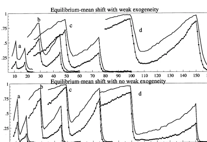
4.3.Equilibrium-mean shift
Experiments in (3) show the contrasting ease of detecting equilibrium-mean breaks. Fig. 5 confirms the anticipated outcomes for the mean shifts: the break-point test rejection frequencies are close to their nominal size of 5% under the null; the break in the equilibrium mean is easily detected, even at quite small sample
Fig. 4. Constancy-test rejection frequencies for loss of cointegration.
sizes, especially when the EqCM enters both relations, which also serves to sharpen the location of the break. Because the relative positions of the breaks are held fixed, the power only increases slowly at p=0.05 as T grows, but has a more marked effect on p=0.01: larger samples do not ensure higher power for detecting the breaks.
To emphasize the detectability issue, note that the corresponding VAR here has the sameG as Eq. (16) throughout, and:
t=
0.11−0.09
changes to t*= 0.14−0.12
. (18)Without the underlying theory to explain this outcome, it might seem astonishing that Eq. (18) can cause massive forecast failure, yet a shift from Eq. (16) to:
G*=
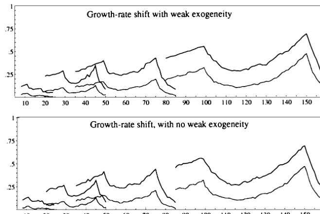
0.80 0.20Finally, experiments in (4) examine the ease of detecting the corresponding doubling of the growth rate. This is a large change in real growth, but that is equivalent to a fraction of the change in (3), and at about 5% rejection, is again almost undetectable on these tests at small T, but now does become increasingly easy to spot as the sample size grows. This is sensible, since the data exhibit a broken trend, but the model does not, so larger samples with the same relative break points induce effects of a larger magnitude. Thus, the type of structural break to be detected affects whether larger samples will help.
The model formulation also matters: if a VEqCM is used, the first growth break shows up much more strongly, as Fig. 7 illustrates. The upper panel shows the break-point test rejection frequencies for the same experiment as Fig. 6; the lower panel records the recursively-computed growth coefficients in the first equation with 92 SE. This increased initial detectability is because the VEqCM ‘isolates’ the shift in g, whereas the VAR ‘bundles’ it with g−am, where the second component can be relatively much larger, camouflaging the shift. Moreover, VAR estimates of g−amgenerally have very large standard errors because of theI(1) representation, whereas estimates of g are usually quite precise. Even so, a large growth-rate change has a surprisingly small effect at T=200 on the recursively-estimated intercept.
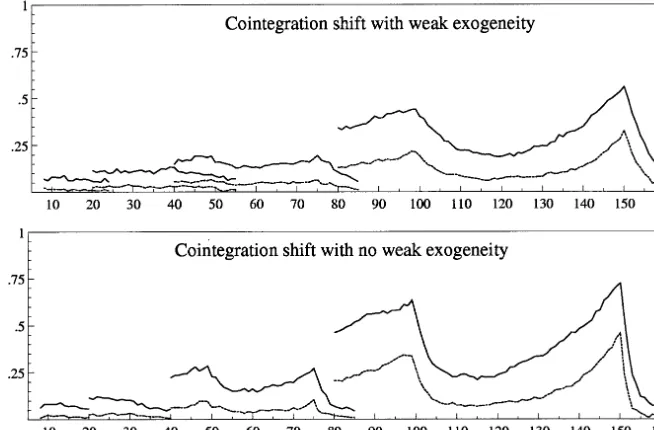
4.5.Cointegration changes
including induced rank changes, and changes to m. The first problem is due to transformations from the class of non-singular matrices H such that a*(b*)%=
aHH−1b
%=ab% under which G is invariant. We have considered the second of
Fig. 6. Constancy-test rejection frequencies for changes ing.
these indirectly above whena changed from a non-zero value to zero, then back. The third requires thatE[(b*)%xt]=m* be known numerically in the Monte Carlo so that the disequilibrium remains at mean zero. In practice, changes in cointegra-tion parameters almost certainly induce changes in equilibrium means, so will be detectable via the latter at a minimum.
The experiment to illustrate this case therefore set m=m*=0, with the other design parameters as before, and changed b% from (1:−1) to (1:−0.9), altering t=g to ensure b%g=0 both before and after the shift, and commencing the simulation fromy%0=(0:0), but discarding the first 20 generated observations. Since the process drifts, power should rise quickly as the sample size grows both because of increased evidence, and the increased data values. Moreover, the re-instatement should be more detectable than the initial change, matching when cointegration is first lost then re-appears. Conversely, the induced change to G is not very large whena%=(−0.1:0):
G=
0.9 0.10.0 1.0
; whereas G*=0.9 0.09 0.0 1.0
,with appropriate changes tot. In one sense, the very small shift inGis remarkably detectable, and reveals how important a role is played by shifts in off-diagonal elements in a VAR: we note with interest that the so-called ‘Minnesota’ prior shrinks precisely these terms towards zero (see Doan et al., 1984). Equally, a slightly bigger change results when a%=(−0.1:0.1), as:
G=
0.9 0.10.1 0.9
; whereas G*=0.9 0.09 0.1 0.91
,and correspondingly, the power is higher in larger samples: see Fig. 8.
5. Potential explanations
Based on the taxonomy of possible sources of forecast errors in Clements and Hendry (1994), Hendry and Doornik (1997) and Clements and Hendry (1998) link the non-detectability to the mean-zero nature of the variables whose parameters are changed. In their taxonomy, some forecasting mistakes derive from parameter changes that multiply the values of the regressors at the forecast origin: when such values are precisely zero, no errors can eventuate. Conversely, other changes multiply the data means (for I(0) components at least) and these only vanish in certain combinations. This suggests that the former, and the appropriate annihilat-ing combinations of the latter, will be hard to detect, and that mean changes will be easy. This matches our simulation results.
Fig. 8. Rejection frequencies for a change in the cointegration parameter.
and dynamics are changed, but the equilibrium mean is constant, and show that the detectability is low. Clements and Hendry (1998) also demonstrate nearly equal detectability from inducing a shift of a given magnitude in the equilibrium mean by either an intercept shift, or by changing the coefficient of a regressor with a non-zero mean, even though the latter involves two sources of change (mean and reaction coefficient) and the former only one. This confirms that changes to reaction coefficients are primarily detectable through the induced mean shift.
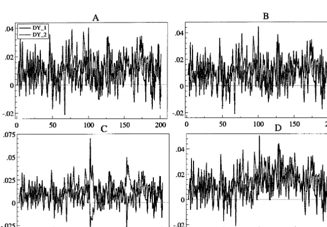
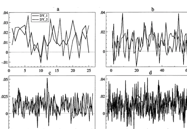
Indeed, the data generated by the constant DGP, and that suffering the shifts shown in Eq. (19), are almost the same, as Fig. 9 (panels a, c) shows, whereas those from Eq. (16) or (4) are noticeably different (panels b, d respectively): bothas are non-zero in every panel. Such a feature is close to a lack of empirical identification, namely the evidence does not discriminate between two very different parameteriza-tions, subject to maintaining the same means, and in fact, similar variances. Changinga only induces variance shifts, and from the data graphs, these are seen to be small relative to the background ‘noise’. Clements and Hendry (1999) derive the variance impacts of changes toa which depend on9aVb(9a)% whereVbis the variance matrix of the cointegrating relations, (b%xt−1−m). When Vb is small, the data resulting from the shift will be only slightly different from the constant DGP, as Fig. 9 shows, despite the substantive change in dynamics. Conversely, the deterministic shift is all too obvious even in data differences (Fig. 10).
Fig. 9. Data generated with and without structural breaks.
Fig. 11. Rejection frequency for a largeashift.
63 D.F.Hendry/Structural Change and Economic Dynamics11 (2000) 45 – 65
G=
0.7 0.30.3 0.7
to G*=0.8 0.2 0.15 0.85
,the rejection-frequency outcomes are shown in Fig. 11, with the corresponding data for the four sample sizes shown in Fig. 12: the break points are far from obvious in the data, and the rejection frequencies remain low, and little improved by the increased sample size.
Finally, the algebra of the intercept in Eq. (3) also helps account for the outcomes in (4). There are two components tot in a VAR, namely the uncondi-tional growth rate,g, and the equilibrium mean times the feedback,am. The former is almost inevitably small, whereas the latter can be huge, simply depending on the units of measurement, as discussed above. Often, therefore, tˆ is a large number, with a large standard error, suggesting its value is very uncertain, and hence — but be careful — that it can be changed considerably without much impact on goodness of fit. Certainly, small changes inG. can offset those intˆ when estimating the VAR unrestrictedly, which is what the large standard errors reflect. However, consider estimating the VAR in Eq. (1) to ‘calibrate’ a Monte Carlo: givenG. (to three digits say), roundtˆ to three digits as well when the numbers are of the order of (say) 10.54 (SE=2.1), thereby using 10.5. The result will generate data wholly unlike those from which the VAR was estimated, because the implicit gˆ has been altered from (say) 0.01 to−0.03: instead of growing at about 4% p.a., the economy is vanishing at 12% p.a.2 Equally, orthogonalizing the equilibrium mean and the growth rate (a linear transform within the estimated model, to which it is invariant), can induce a dramatic change in the remaining intercept standard error, to (e.g.) 0.01 (SE=0.004). This helps explain the difficulty of detecting (4), and suggests that growth-rate changes will be far easier to detect in VEqCMs than VARs. Con-versely, the VAR is more robust to such shifts from the perspective of forecast failure. Finally, we have already explained why relatively tiny VAR parameter changes are readily detected when they correspond to shifts in cointegrating vectors.
6. Conclusion
WithI(1) data generated from a cointegrated VAR, the detectability of a change is not well reflected by the original VAR parameterization. Apparently large shifts in both the VAR intercept and dynamic coefficient matrix need not be detectable, whereas seemingly tiny changes can have a substantial and easily detected effect. Viewing the issue through a vector equilibrium-correction parameterization helps clarify this outcome. Moreover, it reveals that equilibrium mean shifts are readily detectable, whereas mean-zero shifts are not. Thus, the implicit variation-free assumptions about parameters are crucial in a world of structural shifts, with consequential benefits of robustness in forecasting, versus drawbacks of non-detec-tion in modelling. Other tests, including monitoring and variance-change tests,
merit consideration, but overall the results suggest a focus on mean shifts to detect changes of concern to macro-economic forecasting.
Acknowledgements
Financial support from the UK Economic and Social Research Council under grant R65237500 is gratefully acknowledged. I am pleased to acknowledge helpful comments from Mike Clements, Bronwyn Hall, Grayham Mizon, John Muellbauer, Bent Nielsen and Ken Wallis.
References
Anderson, T.W., 1984. An Introduction to Multivariate Statistical Analysis, 2nd. Wiley, New York. Anderson, G.J., Mizon, G.E. (1983). Parameter constancy tests: old and new. Discussion Paper in
Economics and Econometrics, no. 8325, Economics Department, University of Southampton. Anderson, G.J., Mizon, G.E., O’Brien, R.J. (1993). Testing for parameter constancy in systems ofI(0)
variables. mimeo. European University Institute, Florence, Italy.
Brown, R.L., Durbin, L., Evans, J.M., 1975. Techniques for testing the constancy of regression relationships over time. J. R. Stat. Soc. B 37, 149 – 192.
Chow, G.C., 1960. Tests of equality between sets of coefficients in two linear regressions. Econometrica 28, 591 – 605.
Clements, M.P., Hendry, D.F., 1994. Towards a theory of economic forecasting. In: Hargreaves, C. (Ed.), Non-stationary Time-series Analysis and Cointegration. Oxford University, Oxford, pp. 9 – 52. Clements, M.P., Hendry, D.F. (1998). On winning forecasting competitions in economics. Mimeo,
Institute of Economics and Statistics, University of Oxford.
Clements, M.P., Hendry, D.F., 1999. Forecasting non-stationary economic time series. MIT Press, Cambridge, MA.
Doan, T., Litterman, R., Sims, C.A., 1984. Forecasting and conditional projection using realistic prior distributions. Econom. Rev. 3, 1 – 100.
Doornik, J.A. (1996). Object-Oriented Matrix Programming using Ox. International, Timberlake Consultants, London and http://www.nuf.ox.ac.uk/users/doornik, Oxford
Doornik, J.A., Hendry, D.F., 1997. Modelling Dynamic Systems using PcFiml 9 for Windows. Timberlake Consultants, London.
Doornik, J.A., Hendry, D.F., 1998. Monte Carlo simulation, using PcNaive for Windows. Unpublished typescript, Nuffield College, University of Oxford.
Doornik, J.A., Hendry, D.F., Nielsen, B., 1998. Inference in cointegrated models: UK M1 revisited. J. Econ. Surv. 12, 533 – 572.
Engle, R.E., Hendry, D.F., Richard, J.F., 1983. Exogeneity. Econometrica 51, 277 – 304. Reprinted in (a) Hendry, D.E., 1993. Econometrics. Alchemy or Science? Blackwell, Oxford. (b) Ericsson, N.R., Irons, J.S. (Eds.), 1994. Testing Exogeneity. Oxford University, Oxford.
Ericsson, N.R., Hendry, D.E, Prestwich, K.M., 1998. The demand for broad money in the United Kingdom, 1878 – 1993. Scand. J. Econ. 100, 289 – 324.
Hendry, D.F., 1994. HUS revisited. Oxf. Rev. Econ. Policy 10, 86 – 106.
Hendry, D.F., 1997. The econometrics of macro-economic forecasting. Econ. J. 107, 1330 – 1357. Hendry, D.F., Doornik, J.A., 1997. The implications for econometric modelling of forecast failure.
Scott. J. Polit. Econ. 44, 437 – 461.
Hylleberg, S., Mizon, G.E., 1989. Cointegration and error correction mechanisms. Econ. J. 99, 113 – 125 Supplement.
Hylleberg, S., Mizon, G.E., O’Brien, 1993. Testing for parameter constancy in systems of cointegrated variables. Mimeo, European University Institute, Florence.
Rao, C.R., 1952. Advanced Statistical Methods in Biometric Research. Wiley, New York. Rao, C.R., 1973. Linear Statistical Interference and its Applications, 2nd. Wiley, New York.