Analysis of T RFLP data using analysis o

(1)

Other uses, including reproduction and distribution, or selling or

licensing copies, or posting to personal, institutional or third party

websites are prohibited.

In most cases authors are permitted to post their version of the

article (e.g. in Word or Tex form) to their personal website or

institutional repository. Authors requiring further information

regarding Elsevier’s archiving and manuscript policies are

encouraged to visit:

(2)

Analysis of T-RFLP data using analysis of variance and ordination methods:

A comparative study

S.W. Culman

a,

⁎

, H.G. Gauch

a

, C.B. Blackwood

b

, J.E. Thies

a a_{Department of Crop and Soil Sciences, Cornell University, Ithaca, NY, United States}

b

Department of Biological Sciences, Kent State University, Kent, OH, United States

A B S T R A C T

A R T I C L E I N F O

Article history:

Received 5 March 2008

Received in revised form 23 April 2008 Accepted 29 April 2008

Available online 16 May 2008

Keywords:

T-RFLP AMMI PCA DCA CA NMS Sorensen Jaccard Euclidean Ordination Statistical comparison ANOVA

Variation Beta diversity Interaction T-REX

The analysis of T-RFLP data has developed considerably over the last decade, but there remains a lack of consensus about which statistical analyses offer the best means forﬁnding trends in these data. In this study, we empirically tested and theoretically compared ten diverse T-RFLP datasets derived from soil microbial communities using the more common ordination methods in the literature: principal component analysis (PCA), nonmetric multidimensional scaling (NMS) with Sørensen, Jaccard and Euclidean distance measures, correspondence analysis (CA), detrended correspondence analysis (DCA) and a technique new to T-RFLP data analysis, the Additive Main Effects and Multiplicative Interaction (AMMI) model. Our objectives were i) to determine the distribution of variation in T-RFLP datasets using analysis of variance (ANOVA), ii) to determine the more robust and informative multivariate ordination methods for analyzing T-RFLP data, and iii) to compare the methods based on theoretical considerations. For the 10 datasets examined in this study, ANOVA revealed that the variation from Environment main effects was always small, variation from T-RFs main effects was large, and variation from T-RF × Environment (T × E) interactions was intermediate. Larger variation due to T × E indicated larger differences in microbial communities between environments/ treatments and thus demonstrated the utility of ANOVA to provide an objective assessment of community dissimilarity. The comparison of statistical methods typically yielded similar empirical results. AMMI, T-RF-centered PCA, and DCA were the most robust methods in terms of producing ordinations that consistently reached a consensus with other methods. In datasets with high sample heterogeneity, NMS analyses with Sørensen and Jaccard distance were the most sensitive for recovery of complex gradients. The theoretical comparison showed that some methods hold distinct advantages for T-RFLP analysis, such as estimations of variation captured, realistic or minimal assumptions about the data, reduced weight placed on rare T-RFs, and uniqueness of solutions. Our results lead us to recommend that method selection be guided by T-RFLP dataset complexity and the outlined theoretical criteria. Finally, we recommend using binary or relativized peak height data with soil-based T-RFLP data for ordination-based exploratory microbial analyses.

1. Introduction

Terminal restriction fragment length polymorphism (T-RFLP) analy-sis is a robust and effective DNA-fingerprinting technique commonly used to compare microbial communities (Clement et al., 1998, Liu et al., 1997, Osborn et al., 2000, Thies, 2007, Tiedje et al., 1999). Although the analysis of T-RFLP data has developed considerably over the last decade, there remains a lack of consensus about which statistical analyses offer the best means forfinding trends in these data. Researchers surveying recent literature on T-RFLP analyses willfind publications with common research objectives that use a wide range of statistical techniques, often with no justification of their selected method.

In this study, we aimed to address this lack of consensus by comparing the more common ordination methods used in the literature—Principal Components Analysis (PCA), Nonmetric Multi-dimensional Scaling (NMS, MDS, NMDS) with either Sørensen, Jaccard or Euclidean distance, Correspondence Analysis/Reciprocal Averaging (CA) and Detrended Correspondence Analysis (DCA). The utility of a technique new to T-RFLP data analysis, the Additive Main Effects and Multiplicative Interaction (AMMI) model (Gauch, 1992), was also examined.

Blackwood et al. (2003)compared several T-RFLP datasets using two classification methods with several distance measures. Here, we explore another class of methods commonly employed to analyze T-RFLP data. We focused on ordination methods used for exploratory purposes only, not including analyses which test specific hypotheses (e.g. that two microbial communities are signi_ficantly different), or relate microbial community data to environmental variables (i.e., constrained ordinations, such as canonical correspondence analysis).

⁎ Corresponding author. 515 Bradﬁeld Hall, Cornell University, Ithaca, NY 14853, United States. Tel.: +1 607 255 8496; fax: +1 607 255 8615.

E-mail address:swc25@cornell.edu(S.W. Culman).

Contents lists available atScienceDirect

Journal of Microbiological Methods

(3)

The objectives of this study were i) to determine the distribution of variation in a variety of T-RFLP datasets using analysis of variance (ANOVA) ii) to determine the more robust and informative multi-variate ordination methods for exploratory analysis of T-RFLP data and iii) to compare the methods based on theoretical considerations.

2. Materials and methods

2.1. T-RFLP datasets

Ten T-RFLP datasets were used in this study (Table 1). Here we use the word _‘dataset_’ to de_ﬁne a particular microbial community characterized. Each dataset consisted of multiple data matrices which were derived from the same template DNA and reﬂected the same community. Multiple data matrices resulted from 1) the three ways to represent T-RFLP data (binary [i.e., presence/absence], peak height, peak area; called‘types of data’henceforth) and 2) the use of multiple restriction enzymes. We examined 46 data matrices in all, derived from these 10 datasets.

The prairie dataset (Culman, unpublished data) was generated with the same procedures (PCR reactions, restriction enzyme digests, 3730 ABI capillary sequencer) as described inCulman et al. (2006); the alternating wetting and drying (AWD) dataset (Sooksa-nguan et al., unpub. Ph.D. Thesis, Suranaree University of Technology, 2007) was generated with the same procedures described by Lueders and Friedrich (2000), with minor modiﬁcations. Other datasets have been previously described (Table 1). These soil microbial community-based datasets were selected to represent substantial diversity in dataset sizes, targeted microbial communities, imposed treatments and geographical regions.Table 2provides additional detail about the dataset properties and characteristics.

2.2. Data processing

Data processing (determining _‘true peaks_’ from noise, manual alignment of peaks, data transformations, etc.) was performed in numerous ways based on the researcher's original methods. Although the effects of processing raw data were not examined here,Abdo et al. (2006)offer a number of good suggestions to consider in this regard. All T-RFLP electropherograms were visually inspected to ensure quality runs. Electropherograms were tabulated in either GeneScan or Genemapper v3.5 (Applied Biosystems, Foster City, CA) using the Local Southern method as the size-calling algorithm. A baseline threshold of 50 ﬂuorescence units was used to determine ‘true peaks’ from background noise with all datasets, except from the solarization study (Khum and Ramp Bacteria and Fungi), in which the baseline was set at 200. T-RFs less than 50 base pairs (bp) and greater than 500 bp were eliminated from all datasets. Manual alignment of peaks (also

called‘binning’) is often used to account for T-RF drift (improperly sized T-RFs due to differences in fragment migration and purine content [Kaplan and Kitts, 2003, Marsh, 2005]). The Bioreactor, Fractionation '98, Fractionation '99 and Multiregional datasets were all manually aligned (with sample identities concealed). The peaks of the remaining datasets were aligned by rounding to the nearest integer (nucleotide) size.

Raw peak height and raw peak area were relativized to account for uncontrolled differences in the quantity of DNA between samples. Relativized peak height was calculated by dividing each raw peak height by the cumulative peak height of that sample. This is analogous to making each peak height a percentage of the total peak height of a sample. Likewise, relativized peak area was calculated by dividing each raw peak area by the cumulative peak area of that sample. Peak areas from four of the ten datasets could not be obtained.

2.3. Sources of variation in T-RFLP datasets

Multivariate T-RFLP data analysis often begins by organizing the data into a species (T-RF) × samples matrix, analogous to those found in many other applications in community ecology. This matrix will contain three distinct sources of variation: i) main effects for T-RFs, also called operational taxonomic units (OTUs); ii) main effects for Environments (E), also called treatments, plots, samples, and iii) interaction effects for T-RF × Environment (T × E). When this matrix is subjected to a dimensionality-reduction method, the selected method will generally analyze all three sources of variation simultaneously. However, here we argue that when T-RFLP is used as a tool for ex-ploratory microbial community analysis, the scientiﬁcally interesting question commonly being asked is,“How are the T-RFs differentially responding to (i.e. interacting with) the environments?”It is therefore important to distinguish between these sources of variability, and to focus on the T × E interactions.

T-RF variation arises from the fact that some T-RFs occur com-monly across all samples in a dataset, while others occur only rarely. In other words, it reﬂects variability in the means of different T-RFs. When studying macroorganisms, species have a real and tangible meaning to the researcher. On the contrary, for T-RFs, the represented

‘species_’, are often considered somewhat of a _‘black-box_’ during the analysis of T-RFLP datasets. Microbial ecologists must use caution when conceptualizing T-RFs as unique species or even unique OTUs, as Clement et al. (1998) and others have shown that multiple organisms can share similar or identically-sized T-RFs. Except when working with a speciﬁc organism, group-speciﬁc primers or with a locally-constructed clone library, individual T-RFs in a T-RFLP dataset are often ambiguous, limiting the researcher from drawing information from them. T-RF variation constitutes inherently simple information on commonness or rareness that can distract a

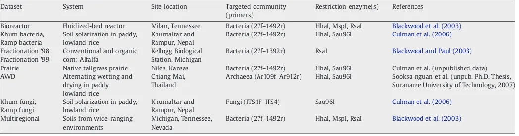
Table 1

T-RFLP datasets used in this study

Dataset System Site location Targeted community

(primers)

Restriction enzyme(s) References

Bioreactor Fluidized-bed reactor Milan, Tennessee Bacteria (27f–1492r) HhaI, MspI, RsaI Blackwood et al. (2003)

Khum bacteria,

Bacteria (27f–1492r) HhaI, Sau96I Culman et al. (2006)

Fractionation '98

Bacteria (27f–1392r) RsaI Blackwood and Paul (2003)

Prairie Native tallgrass prairie Niles, Kansas Bacteria (27f–1492r) HhaI, Sau96I Culman et al. (unpublished data)

AWD Alternating wetting and

drying in paddy lowland rice

Chiang Mai, Thailand

Archaeea (Ar109f–Ar912r) HhaI, Sau96I Sooksa-nguan et al. (unpub. Ph.D. Thesis, Suranaree University of Technology, 2007)

Khum fungi,

Fungi (ITS1F–ITS4) Sau96I Culman et al. (2006)

Multiregional Soils from wide-ranging environments

Michigan, Tennessee, Nevada

Bacteria (27f–1492r) HhaI, MspI, RsaI Blackwood et al. (2003)

(4)

multivariate analysis from capturing the truly complex interaction information.

The logic outlined above for T-RF variation does not apply to the E variation in a T-RFLP data matrix, which arises from differences in numbers of peaks or overall signal strength in T-RFLP profiles representing different environments. Environments represent a very real and tangible concept to the researcher. However, true E variation (e.g., due to microbial biomass) is masked in T-RFLP analyses by analytical variability related to, for example, DNA puri_fication efficiency, pipetting error, and community structure (Blackwood et al., 2003, Dunbar et al., 2001). As a result, this known source of analytical noise is commonly removed in peak height and area with the relativization process. Hence, when using T-RFLP as a method of exploratory data analysis on microbial community structure, the T × E variation is often most relevant to the researcher. In this study, we discuss sources of T-RFLP variation in this context, assuming that T × E variation is of primary interest.

2.4. Analysis of variance

Two-way ANOVA was performed on all T-RFLP datasets in Table 1, using MATMODEL software (Gauch, 2007, Gauch and Furnas, 1991). The percent of variation from each source in the ANOVA (T-RF, E, and T × E) was calculated by dividing that source's sum of squares (SS) by the treatment SS and multiplying by 100. The interaction SS was further decomposed into interaction signal SS and interaction noise SS. The interaction noise SS was estimated by multiplying the interaction degrees of freedom (df) by the mean squared error (MSE). The interaction signal SS was estimated by subtracting the interaction noise SS from the interaction (total) SS. The interaction signal SS and interaction noise SS were then divided by the treatment SS to calculate the percent variation in the dataset due to these sources. See

Gauch (1992)for more details on these calculations.

2.5. Empirical testing of ordination methods

In order to determine the more robust and informative methods, several of the more common multivariate statistical ordination analyses in the literature were compared: (i) PCA, (ii) CA, (iii) DCA and (iv) NMS using the Sørensen (Bray_–Curtis) distance measure, (v) NMS using the Jaccard distance measure, (vi) NMS using the Euclidean distance measure, and (vii) AMMI. The AMMI model, also known as

‘doubly-centered PCA_’, has been used extensively in agricultural research, particularly in analyses of yield trials. AMMI uses ANOVA to

ﬁrst partition the variation into main effects and interactions, and then applies PCA to the interactions to create interaction principal components (IPCs) (Gauch, 1992). Therefore, instead of examining overall variability of the data, AMMI can focus on the differential responses of T-RFs to the environments/ treatments, that is, T × E. Here, the_‘main effects_’are deﬁned as the T-RF and E variation. Including the AMMI model, there were 7 separate analyses performed on each of the 46 T-RFLP data matrices, totaling 322 graphs evaluated.

Environments were replicated for all experiments in this study. Initially, two analyses of each statistical method were run on each dataset, one analysis with the original replicated dataset and a second analysis with the averages over replicates, using T-REX

software (Culman et al., unpublished;http://trex.biohpc.org/). The two ordinations produced from these analyses were very similar, and if the two graphs were overlaid, the individual replicates would simply scatter somewhat around the averaged value. The two ordinations were equally discriminatory with respect to our criteria for evaluating statistical methods (see below), so we subsequently focused the comparison on the simpli_ﬁed datasets with averages over replicates.

2.6. Statistical software and parameters

• PCA was performed with PC-ORD v4 (MjM Software Design, Gleneden Beach, OR;McCune and Mefford, 1999) with the Variance/Covariance (centered) option selected. This option centers the T-RFs by subtract-ing the average for each RF over E from each matrix entry for that T-RF. This produces a variance–covariance matrix. By contrast, the use of the Correlation (standardized) option_ﬁrst centers the T-RFs and then divides each matrix entry by the standard deviation for each T-RF, thus producing a correlation matrix. Our reason for this selection is discussed in Section 3.3.5.

• CA was performed with PC-ORD, with Downweight rare species not selected.

• DCA was performed with PC-ORD using the default settings: (i) Downweight rare species was not selected, (ii) Rescale axes was selected, (iii) Rescaling threshold = 0, and (iv) Number of segments = 26.

• NMS was performed with PC-ORD, using the Medium Autopilot mode. This mode speciﬁes: (i) Maximum number of iterations = 200, (ii) Instability criterion = 0.0001, (iii) Starting number of axes = 4, (iv) Number of real runs = 15, and (v) Number of randomized runs = 30. Three separate distance measures were selected for the NMS analysis: Sørensen, Jaccard and Euclidean. When the Autopilot

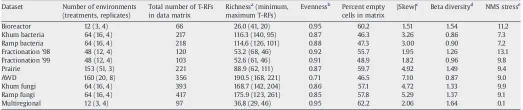
Table 2

Characteristics of T-RFLP datasets used in this study

Dataset Number of environments

Khum bacteria 64 (16, 4) 217 116.3 (140, 95) 0.87 46.3 3.26 0.86 7.3

Ramp bacteria 64 (16, 4) 218 114.6 (126, 101) 0.88 47.3 3.00 0.90 7.2

Fractionation '98 48 (12, 4) 120 53.2 (68, 46) 0.92 55.7 1.95 1.26 13.1

Fractionation '99 48 (12, 4) 103 52.6 (61, 46) 0.91 48.9 1.82 0.96 9.8

Prairie 153 (51, 3) 221 88.9 (62, 111) 0.87 59.7 4.92 1.49 9.4

AWD 160 (20, 8) 356 190.5 (168, 221) 0.71 46.5 7.10 0.87 9.0

Khum fungi 64 (16, 4) 393 168.7 (142, 204) 0.86 57.1 4.72 1.33 9.9

Ramp fungi 64 (16, 4) 417 175.9 (123, 261) 0.85 57.8 5.29 1.37 9.1

Multiregional 12 (3, 4) 97 36.8 (29, 46) 0.95 62.2 2.06 1.64 0.1

For experiments with multiple restriction enzymes, values were averaged across those enzymes. Since skew and NMS stress varied between types of data, these values were averaged over all types of data and enzymes.

a

Deﬁned as the average number of T-RFs in a dataset. b _{Pielou's J.}

c _{|Skew|values averaged over binary data, relativized peak height and relativized peak area were 0.8, 4.8, and 6.8, respectively.} d

Deﬁned as: [(total number of T-RFs in a dataset) / (average T-RF richness in the environments)]−1. e

(5)

mode recommended aﬁnal solution that was more or less than 2 axes, the analysis was re-run with the same parameters, but forcing a 2-dimensional solution (Autopilot mode deselected).

• The AMMI analysis was performed with MATMODEL.

Scatterplots of theﬁrst two axes of each ordination were graphed with Minitab v.14.1 (State College, PA).

2.7. Criteria for empirical comparisons

Evaluating the ability of an ordination to reveal the true structure of a dataset is problematic, because it is only with simulated data that we know the true and exact structure of a particular dataset. However, with_ﬁeld data, we do have two considerations to aid our evaluation of the accuracy and effectiveness of an ordination: (i)a

priori information about the experiment's treatment design and

microbial community dynamics and (ii) consensus among the ordinations performed. In this study we used these two criteria as a surrogate for the true structure of the data. For each of the 46 data matrices, we compared the scatterplots of theﬁrst two axes produced by the seven ordination methods and evaluated each method's ability to demonstrate known gradients or treatments, such as time, crop phenology, soil depth, etc. We also examined each method's per-formance against one another within each data matrix, evaluating if the method complied with the consensus reached by the majority of analyses. For each data matrix, every method was scored as demonstrating the expected gradient/s either i) very well, ii) reasonably well or iii) poorly/not at all. In addition, the method was scored as reaching a general consensus with the other methods or not. Consensus could be viewed as a more robust ranking scheme, indicating if the overall interpretation of a particular ordination was similar to the majority of analyses. The ranking of ordination methods was judged for consistency across all datasets to minimize any anomalous results speci_ﬁc to a given dataset. The large number of datasets examined here mitigated the subjectivity of this coarse scoring system, making this empirical assessment more robust than in any previous study.

2.8. Most informative type of data

The most informative type of data (binary, relativized peak height or relativized peak area) was evaluated based on the number of times a consensus with the majority of the methods was reached. The total number of times a consensus was reached was summed over every data matrix for that type of data.

2.9. Theoretical criteria for evaluating methods

The ordination methods in this study were not only compared empirically, but also theoretically. Although these criteria are not exhaustive, the more relevant theoretical aspects when analyzing T-RFLP data are listed below:

1) Assumptions—What assumptions does the analysis make about the data? Are these assumptions appropriate for microbial community data?

2) Proportion of variation represented—Does the analysis quantify the amount of variation captured in theﬁrst 2 (or 3) axes?

3) Integrated dual analysis_—Is there an integrated analysis of T-RFs and environments, or only an analysis of one of these?

4) Uniqueness of solution—Given the same data, would multiple users come to similar conclusions? Or does this method suffer from

‘optionitis’? (‘Optionitis’ = an excessive number of choices not determined by objective criteria).

5) Weight of rare T-RFs—How much importance does the analysis give rare T-RFs?

3. Results

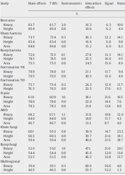
3.1. Analysis of variance

Table 3 shows the distribution of variation within the T-RFLP datasets from ANOVA, arranged in descending order of variation due to main effects (T-RF and E variation). Main effects variation ranged from 89.4% (Bioreactor, relativized peak height) to 39.4% (Multi-regional soil, binary). The vast majority of the main effects variation was made up of T-RF variation, with E variation contributing very little. Note that E main effects with relativized peak height and area will be exactly zero, as a result of the relativization process. However, E main effects of binary data, which were not relativized, still contributed no more than 2.0% (Bioreactor) and as little as 0.1% (Ramp Bacteria and Fractionation '98) of the total variation. This indicates that the total number of T-RFs in each sample was nearly constant.

Percentages of variation due to interaction effects and the relative proportion of interaction signal not only varied with the dataset, but this variation coincided with background knowledge of these datasets. For example, the Bioreactor dataset is composed of bacterial communities from several bioreactors that were treated identically.

Table 3

Percent of variation in T-RFLP datasets from analysis of variancea

Study Main effects T-RFs Environments Interaction

effects

Signal Noise

%

Bioreactor

Binary 83.7 81.7 2.0 16.3 6.3 10.0

Height 89.4 89.4 0.0 10.6 6.2 4.4

Khum bacteria

Binary 73.7 73.4 0.3 26.3 12.2 14.1

Height 83.4 83.4 0.0 16.6 6.8 9.8

Area 84.8 84.8 0.0 15.2 6.9 8.3

Ramp bacteria

Binary 72.6 72.5 0.1 27.4 13.3 14.1

Height 74.5 74.5 0.0 25.5 16.0 9.5

Area 75.5 75.5 0.0 24.5 15.6 8.9

Fractionation‘98

Binary 78.9 78.8 0.1 21.1 11.7 9.4

Height 79.5 79.5 0.0 20.5 15.6 4.9

Fractionation‘99

Binary 75.7 75.4 0.3 24.3 12.6 11.7

Height 76.5 76.5 0.0 23.5 17.0 6.5

Prairie

Binary 61.9 60.9 1.0 38.1 21.6 16.5

Height 78.0 78.0 0.0 22.0 14.4 7.6

Area 78.2 78.2 0.0 21.8 13.8 8.0

AWD

Binary 68.2 67.1 1.1 31.8 19.8 12.0

Height 84.0 84.0 0.0 16.0 11.7 4.3

Area 86.7 86.7 0.0 13.3 8.7 4.6

Khum fungi

Binary 60.1 59.3 0.8 39.9 14.7 25.2

Height 60.3 60.3 0.0 39.7 21.6 18.1

Area 59.4 59.4 0.0 40.6 21.9 18.7

Ramp fungi

Binary 52.9 51.0 1.9 47.1 21.0 26.1

Height 54.4 54.4 0.0 45.6 32.0 13.6

Area 53.5 53.5 0.0 46.5 32.8 13.7

Multiregional

Binary 39.4 39.1 0.3 60.6 56.6 4.0

Height 46.5 46.5 0.0 53.5 52.2 1.3

a

The values are percentages based on the three T-RFLP data types: binary (presence/ absence), height (relativized peak height) and area (relativized peak area). Main effects and interaction effects make up the two main sources of variation within a T-RFLP dataset. The main effects are a subtotal for the T-RFs and Environments. Similarly, the interaction effects are a subtotal for both interaction signal and interaction noise. For experiments with multiple restriction enzymes, the variation across these enzymes was averaged, as this variation was insigniﬁcant.

(6)

These bacterial communities would be expected to vary little, and the ANOVA conﬁrms this expectation, with the interaction effects making up only 16.3% and 10.6% of the total variation in the binary and peak height data, respectively. Of this variation, just 6% is from interaction signal for both types of data. In contrast, the Multiregional soil dataset is composed of communities from extremely different soil types. These communities appear to be very different, as the majority of the total variation in the binary and peak height data is due to interaction signal (56.6% and 52.2%, respectively). The ANOVA output given in

Table 3 suggests that the community differences need not be that extreme in order to be detected. Relatively larger interaction variation from the Khum and Ramp fungal datasets compared to the Khum and Ramp bacterial datasets also coincides with the results of the ordinations reported elsewhere (Culman et al., 2006).

ANOVA revealed overall consistency in the distribution of variation between the three types of data: binary, relativized peak height and relativized peak area (Table 3). Analyzing binary data resulted in the lowest main effects variation and the highest interaction effects variation in 9 out of the 10 datasets. The ratio of interaction signal to noise was lowest in the binary data 9 out of 10 times and highest in peak height 7 out of 10 times.

3.2. Empirical ordination results

Overall, the ordinations from the seven analyses generally yielded graphs that did not drastically deviate from one another. Conse-quently, the scoring differences were limited to a relatively narrow range (Table 4). Individual methods are discussed below.

3.2.1. PCA and AMMI

In this study, both variable-centered (T-RF-centered) PCA and AMMI (doubly-centered PCA) were performed. In T-RF-centered PCA, the T-RF main effects variation is reduced to zero in a manner similar to the relativization process with the environments. Hence, with little to no main effects variation, a T-RF-centered PCA approximates the AMMI analysis, because the E variation is small (2% or less). As a result, the T-RF-centered PCA and AMMI analysis ordinations were nearly identical and performed equally well at recovering expected gradients, reaching a consensus with every data matrix analyzed (Table 4).

Variants of PCA that were not T-RF-centered or T-RF-standardized did not remove the T-RF main effects variation and as a result produced quite different ordinations that were dominated by T-RF main effects.

Fig. 1a shows the results of an environment-centered PCA, an analysis that removes variation that is already very small (0.8% E main effects), but does nothing to remove the main source of variation (59.3% T-RF main effects).Fig. 1b shows PCA (AMMI) applied to the same data, but after ﬁrst removing the large T-RF variation and small E variation. Removing these sources of variation (i.e., doubly-centering) produces the interaction matrix that AMMI ordinates. The environment-centered PCA (Fig. 1a) is an inferior procedure, as the more subtle trends in treatment difference (indicated by circled data points) are not consistently captured. This analysis could be produced by a researcher simply entering and analyzing a mistakenly transposed T-RFLP data matrix. Note that a variable-centered PCA is the default procedure in some statistical packages (e.g., SAS, Cary, NC), while in other commonly used packages (e.g., Canoco, Microcomputer Power, Ithaca, NY), the user must select this option.

3.2.2. CA and DCA

CA was among the poorer methods for demonstrating expected gradients and reaching a consensus with the other methods (Table 4). However, when CA was re-run with rare species down-weighted with four of the data matrices, the resulting ordinations were acceptable and reached a consensus with other methods, making the method more robust (data not shown). DCA performed comparable to other methods with all datasets, except the Multi-regional dataset, where it scored _‘reasonably well_’ in all six of the data matrices. These did not affect the overall interpretation of the dataset, enabling DCA to reach a consensus with all 46 data matrices, demonstrating its overall robustness (Table 4).

Table 4

Results of empirical comparisons between ordination methods

Demonstrated known gradient(s)

Method Very well Reasonably

well

Poorly or not at all

Reached consensus with other ordinations

AMMI 25 21 0 46

T-RF centered PCA 25 21 0 46

CA 21 19 6 42

DCA 23 23 0 46

NMS with Sørensen 26 18 2 44

NMS with Jaccard 25 20 1 45

NMS with Euclidean 22 20 4 42

(7)

3.2.3. NMS

Overall, the ordinations produced from NMS analyses were very similar to the eigenvector-based methods evaluated above. NMS analyses with Sørensen and Jaccard distance measures scored high in demonstrating gradients _‘very well_’, with the Sørensen distance measuring scoring better than any method compared (Table 4). However, two NMS analyses with Sørensen distance and one analysis with the Jaccard distance measure produced ordinations that were wildly different from the consensus reached by other ordinations. These analyses were re-run several times each with different initial conﬁgurations, but produced similar idiosyncratic results. NMS with the Euclidean distance measure ranked the worst at reaching a consensus and was judged to be the poorest performing method examined (Table 4).

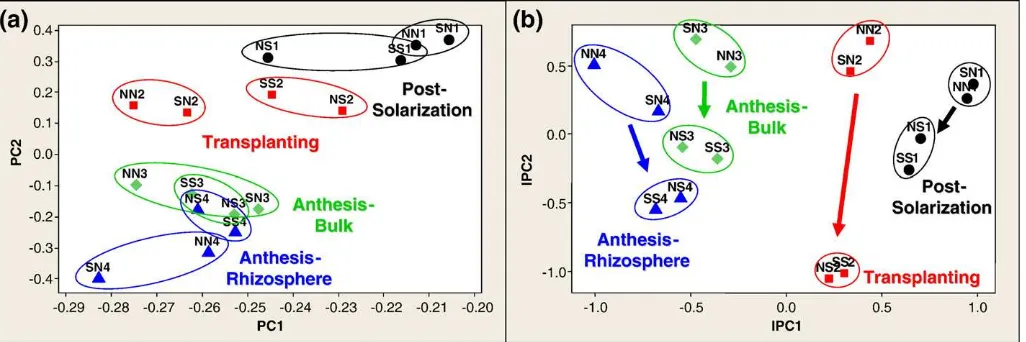
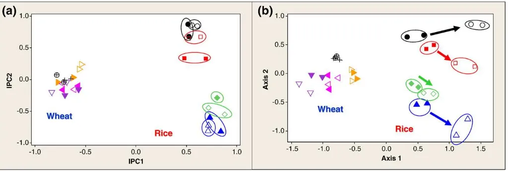
For the most complex datasets, NMS analyses with Sørensen and Jaccard distance measures performed better at demonstrating known gradients than all other analyses. For example, NMS outperformed all other analyses with the entire tallgrass prairie datasets analyzed as a whole, but when this dataset was decomposed (based on experi-mental design) into two separate datasets and reanalyzed, the NMS analyses were no longer more discriminatory than the other methods (data not shown). This phenomenon was also observed in the datasets from the solarization study (Fig. 2). The combined rice and wheat dataset (Ramp, Bacteria,Sau96I enzyme) is shown analyzed with the AMMI model (Fig. 2a) and with NMS with the Sørensen distance measure (Fig. 2b). When the rice and wheat seasons were analyzed as a single dataset, the NMS analysis was more discriminatory at demonstrating the treatment differences (soil solarization) in rice than was the AMMI analysis. This is demonstrated by the circled data points and arrows inFig. 2b, and the lack of consistency in treatment trends represented inFig. 2a. However, when the rice season was decomposed and analyzed separately from the wheat season (Fig. 3 from Culman et al. (2006)), the resulting ordinations from all the methods were equally informative, and were generally more informative than the NMS analysis of the combined rice and wheat dataset. Neither AMMI nor NMS revealed treatment differences in the wheat sampling periods when either the combined or separated datasets were analyzed.

3.2.4. Most informative type of data—binary, peak height or peak area

Overall, there were few differences in theﬁnal ordinations derived from the three different types of data. Our analyses demonstrated that binary data were the most robust, with only one instance when a

method didn't reach a consensus in the binary data matrices (18 total). A consensus was not reachedﬁve times in the relativized peak height data matrices (18 total), andﬁve times in the relativized peak area data matrices (10 total).

3.3. Theoretical ordination results

3.3.1. Assumptions

PCA uses Euclidean distance and assumes a linear relationship among variables, which may not be appropriate for community ecology data (Beals, 1984, McCune and Grace, 2002). However, this issue can be resolved by the use of appropriate data transformations which allow PCA to be performed with a wide variety of distance metrics appropriate for community ecology data (Legendre and Gallagher 2001). CA and DCA are both eigenvector-based ordination techniques that use a chi-square distance measure and assume that T-RFs have a unimodal distribution along ecological gradients. This is a more appropriate assumption than linearity for ecological community data, as it is in agreement with the usual outcome of ecological studies (Gauch, 1982), but is still capable of being violated with community ecology datasets (Beals, 1984, Legendre and Legendre, 1998, Minchin, 1987). NMS fundamentally differs from the above techniques because it uses rank order information from a similarity matrix to ordinate the data, rather than metric information (Gauch, 1982). NMS does not assume linear relationships among variables and it allows virtually any distance measure to be used in the construction of the similarity matrix.Rees et al. (2004)argued that these attributes make NMS more appropriate for T-RFLP community analysis over other methods.

3.3.2. Proportion of variation represented

Interpretation of ordination analyses must be guided by an objective assessment of how much variation is being captured in the

first few ordination axes. PCA (including AMMI) is the only method that can precisely calculate this variance from the ratio of eigenvalues to total variation. This attribute favors PCA when an objective assessment of variation represented is desired. It should be noted that all methods can use an after-the-fact assessment which calculates a coefficient of determination (r2) as an assessment of how much variation is captured in thefirst few axes (McCune and Grace, 2002). However, this approach was not evaluated here since several distance measures were compared, making these measures incommensurable. The proportion of variation represented in the IPCs in AMMI analysis can be directly related to the predicted interaction signal

Fig. 2.T-RFLP bacterial community data (Ramp,Sau96I, binary) analyzed with (a) AMMI (a) and NMS with Sørensen distance measure, demonstrating the greater discriminatory power of NMS in the rice crop with heterogeneous data (rice and wheat data analyzed together). Closed data points represent non-solarized plots; open data points represent solarized plots. Circled data points represent the rice crop; non-circled data points represent the wheat crop. Differing shapes and colors represent different sampling time periods. SeeCulman et al. (2006)for details of experiment and legend.

(8)

given inTable 3. For instance, the T × E signal comprises only 14.7% of the total variation for the data represented inFig. 1b, but thisfigure focuses on T × E exclusively and AMMI's first two IPCs account for nearly all of the interaction signal. Across all datasets, the average percent of interaction variation represented in the_first two IPCs was 94.5%. This directed focus can be advantageous when research interests focus on T × E, and this interaction is a small portion of the overall variation.

3.3.3. Integrated dual analysis

Biplots are scatterplots of samplesandspecies (E and T-RFs) in the same graph. These can be extremely insightful in determining which T-RFs are most closely associated with which environments. Eigen-vector techniques (PCA, AMMI, DCA, and CA) use integrated, dual analysis of the rows and columns of a data matrix, resulting in scores for both environments and T-RFs. NMS analyses are not dual by nature, because a distance matrix is constructed based on similarities of T-RFsorE, but not both.

3.3.4. Uniqueness of solution

Analyses that have a large number of parameters that need to be speci_ﬁed have potential for confusion.Optionitis—a term we use to describe this phenomenon—can become problematic when these parameters are not selected by objective criteria and when the results vary depending on which parameters are selected. PCA has several variants, but the most appropriate can be selected by objective criteria. CA and DCA have a few important input options that the user must select. Depending on the software used, NMS has several criteria that need to be selected (distance measure, stress level, number of iterations, starting conﬁguration, number of axes), which can lead to a number of possible outcomes. Current computing power enables the user to be very conservative with most of these param-eters, alleviating most of these concerns. However, in our experience, if these parameters are not set conservatively, the results can be quite variable.

3.3.5. Weight of rare T-RFs

The relative inﬂuence of rare T-RFs on the ordination can be determined by the distance measure employed in the analysis. The chi-square distance measure has been criticized by several authors (Faith et al., 1987, Legendre and Legendre, 1998, Minchin, 1987) for its tendency to give greater weight to rare species and less weight to commonly occurring species. This is an important issue as rare T-RFs commonly occur in T-RFLP data and can be methodologically exacerbated with mis-called electrophoretic reads of peak size (T-RF drift) or by PCR artifacts. Since both CA and DCA use the chi-square distance measure, they will potentially give greater weight to rare species—an undesirable characteristic. Although the program DEC-ORANA (Hill, 1979), on which most DCA software is built, and various versions of CA do give the option of downweighting rare species, this does not fully remedy the problem (Jongman et al., 1995). Likewise, rare species are also given greater weight in standardized (correlation-matrix) PCA (not empirically evaluated here) than in centered PCA. Because standardized variables give each T-RF equal variance, rare and common T-RFs contribute equal information to the ordination. Therefore, using T-RF-centered variables, rather than T-RF-standar-dized variables, is generally more desirable in T-RFLP analysis. NMS offers the greatest ﬂexibility with regard to selecting a distance measure.Rees et al. (2004)and others (Legendre and Legendre, 1998, McCune and Grace, 2002) have recommended the Sørensen distance measure (with NMS) as an ecological distance measure for several reasons. Perhaps the most important is the ability of Sørensen to appropriately ignore joint absences (i.e. if two samples do not contain many of the same T-RFs, this is not measured as similarity between them). SeeLegendre and Legendre (1998)for further discussion of these ecological distance measures.

The potential problem of rare species receiving greater weight can be side-stepped by simply deleting rare species from the dataset. While this would not be appropriate if the researcher was interested in diversity measures, it can often reduce overall noise and improve the correlation structure in datasets. McCune and Grace (2002)

suggest deleting species (T-RFs) that only occur in fewer than 5% of the samples. In our experience, deleting rare T-RFs strengthens the observed patterns from ordinations.

4. Discussion

Analysis of variance was performed on all datasets in this study in order to gain insight into the distribution of variation in these T-RFLP datasets. Main effects variation dominated the majority of the datasets and was comprised almost entirely of T-RF variation. This variation is inherently simple information on the rareness or commonness of T-RFs and is often not of primary interest. The main effects variation from E was always small—either the total number of T-RFs across all treatments remained fairly constant (in binary data), or the variation was eliminated by the relativization step (in peak height and area) to remove a known source of analytical noise. The small contribution from E was due in part to the quality control step that eliminated poor-quality runs from the analysis, but also reﬂected the nature of the datasets examined. Despite often large differences between treat-ments, the number of T-RFs in each E remained fairly constant (evenness values inTable 2; binary E variation inTable 3). The nature of T-RFs and E main effects variation directs the researcher to focus entirely on the interaction variation, as nearly all of the relevant information concerning the environments, imposed treatments, samples, etc. is found in the interaction. This interaction captures how T-RFs differentially respond to the E. In this context, ANOVA can be used as a standard procedure that can be applied to any dataset in order to objectively measure microbial community dissimilarity. This in turn can provide insight into whether these differences are ecologically meaningful.

Table 3demonstrates a large proportion of dataset variation from T-RFs. This variation needs to be removed by the selected analysis, or the resulting ordination will be dominated by this simple and often uninteresting information. This phenomenon is demonstrated dra-matically inFig. 1. We were intrigued to discover that the necessity to remove the T-RF variation only seems to be germane with PCA, as all the other methods examined in this study (CA, DCA and NMS) have means to ignore or minimize this variation.

In this study, all methods produced empirical results that generally did not deviate from the overall consensus. Likewise, the theoretical criteria did not solely favor one particular analysis over the others. However all methods did not perform equally. Some methods have distinct advantages which aid in data interpretation and tend to be more robust, while others have qualities that could be potentially problematic.

(9)

experience, soil-based T-RFLP data are generally not very complex relative to other types of ecological community data.Legendre and Gallagher (2001) refer to these types of datasets as having short gradients. Measures of dataset complexity can account for various factors, including sample heterogeneity, the number of underlying gradients, T × E interactions, and relative noise to signal. We found sample heterogeneity (also known as beta diversity) to be a satis-factory and simple measure of this complexity.

We assessed T-RFLP sample heterogeneity by measuring beta diversity, deﬁned as [(total number of T-RFs in a dataset) / (average T-RF richness in the environments)]−1 (Whittaker, 1972). McCune and Grace (2002) state as a rule of thumb that beta diversity less than 1 is rather low and greater than 5 is very high. We found the average beta diversity across all T-RFLP datasets to be 1.22, suggesting that overall heterogeneity between environments in T-RFLP datasets is relatively low. (Note that beta diversity is often highly correlated with the percent of empty cells in a data matrix.) Another observation to support the idea that soil-based T-RFLP data have relatively low complexity was the empiricalﬁndings. Overall, ordinations of the same dataset with different methods did not drastically deviate from each other, suggesting the relative ease of the ordinations by the various methods. This same phenomenon_—when sample heterogeneity is low, ordinations from different methods perform comparably—has been shown in numerous ecological studies (Beals, 1984, Fasham, 1977, Gauch et al., 1977, Kenkel and Orloci, 1986, Minchin, 1987).

The lack of complexity or heterogeneity in T-RFLP datasets is likely related to the type of questions that T-RFLP is employed to ask. Microbial ecologists rarely use T-RFLP to assess community structure from two very different environments (e.g., very wet to very dry gradients, very different soil types, etc.) as most researchers will (often correctly) assume that these microbial communities will be very different. As a consequence, the length of the ecological gradient is often kept relatively short by the researcher's experimental design when employing T-RFLP.

An irony currently exists in the literature in which researchers meticulously report the concentration and reaction details of their PCR (even though T-RFLP has been shown to be robust to these variations (Osborn et al., 2000)), but often fail to report rudimentary information about the statistical analyses. A survey of recent T-RFLP literature will show many papers that fail to report any parameters about the analyses employed, even parameters as fundamental as which variant of PCA or distance measure of NMS. Omissions such as these should be avoided, as they compromise the repeatability of experiments and analyses.McCune and Grace (2002)have offered criteria to report for each analysis. Of these criteria, we judge the most important for T-RFLP analysis to be: i) PCA and AMMI: form of cross-products matrix (correlation, variance–covariance, or doubly-centered), number of axes interpreted and the proportion of variance represented by each axis, and justi_fication of the assumption of linear relationships among T-RFs; ii) CA and DCA: number of axes in-terpreted and the proportion of variance represented by each axis (after-the-fact assessment), whether downweighting was selected, and justification of the assumption of unimodal distribution of T-RFs; iii) NMS: distance measure, stress of final solution, number of dimensions infinal solution, proportion of variance represented by each axis, number of runs with real data, and number of iterations for

ﬁnal solution.

5. Conclusions and recommendations

Based on our ﬁndings there is no single method that we can recommend above all others for soil-based T-RFLP community analysis. We recommend that it become conventional for all T-RFLP data to be reported with two important dataset characteristics: beta diversity and percent of main and interaction effects. We found these two characteristics to be highly informative indicators of the nature of

the datasets examined in this study. Datasets with high beta diversity (2 or greater in our experience), or otherwise greater complexity than those examined in this study, should likely employ NMS analyses with Sorensen or Jaccard (or another appropriate distance measure). Analyses of low beta diversity datasets should be more strongly guided by the outlined theoretical criteria. Both interaction effects and beta diversity are easily calculated with the free online software,

T-REX(http://trex.biohpc.org/).

We prefer the AMMI analysis for most T-RFLP data that we have encountered, as it has performed very well empirically, and also yields an ANOVA table which provides a tool to assess microbial community dissimilarity. The ability of the analysis to focus on the differential responses to the treatments may also be amenable for use on microarray data or other approaches focusing on differential gene responses. Unless otherwise justi_fied, DCA and CA analyses should be run with the ‘downweight rare species’ option selected. We generally do not recommend NMS with the Euclidean distance mea-sure; it performed the worst empirically, and has no advantages over the other methods that we judge important for T-RFLP. Finally, we recommend confirming initial findings with other multivariate method/s whenever possible.

In this study, binary data were less prone to variable results than relativized peak height or area, making binary data the most robust measure. Relativized peak height had, on average, greater interaction signal to interaction noise ratios, lower |skew|, and lower NMS stress than relativized peak area. For these reasons and those outlined in

Grant et al. (2003), we recommend using binary data or relativized peak height for ordination analyses over relativized peak area. Although this study dealt exclusively with T-RFLP data, many of the concepts discussed here are also applicable to microbial community datasets generated by other methods.

References

Abdo, Z., Schuette, U.M.E., Bent, S.J., Williams, C.J., Forney, L.J., Joyce, P., 2006. Statistical methods for characterizing diversity of microbial communities by analysis of terminal restriction fragment length polymorphisms of 16S rRNA genes. Environmental Microbiology 8, 929–938.

Beals, E.W., 1984. Bray–Curtis ordination: an effective strategy for analysis of multivariate ecological data. Advances in Ecological Research 14, 1–55.

Blackwood, C.B., Marsh, T., Kim, S.-H., Paul, E.A., 2003. Terminal restriction fragment length polymorphism data analysis for quantitative comparison of microbial communities. Applied and Environmental Microbiology 69, 926–932.

Blackwood, C.B., Paul, E.A., 2003. Eubacterial community structure and population size within the soil light fraction, rhizosphere, and heavy fraction of several agricultural systems. Soil Biology & Biochemistry 35, 1245–1255.

Clement, B.G., Kehl, L.E., Debord, K.L., Kitts, C.L., 1998. Terminal restriction fragment patterns (TRFPs), a rapid, PCR-based method for the comparison of complex bacterial communities. Journal of Microbiological Methods 31, 135–142. Culman, S.W., Duxbury, J.M., Lauren, J.G., Thies, J.E., 2006. Microbial community

response to soil solarization in Nepal's rice-wheat cropping system. Soil Biology & Biochemistry 38, 3359–3371.

Dunbar, J., Ticknor, L.O., Kuske, C.R., 2001. Phylogenetic speciﬁcity and reproducibility and a new method for analysis of terminal restriction fragment proﬁles of 16S rRNA genes from bacterial communities. Applied And Environmental Microbiology 67, 190–197.

Faith, D.P., Minchin, P.R., Belbin, L., 1987. Compositional dissimilarity as a robust measure of ecological distance. Plant Ecology 69, 57–68.

Fasham, M.J.R., 1977. A comparison of nonmetric multidemensional scaling, principal components and reciprocal averaging for the ordination of simulated coenoclines and coenoplanes. Ecology 58, 551–561.

Gauch, H.G., 1982. Multivariate Analysis in Community Ecology. Cambridge University Press, Cambridge.

Gauch, H.G., 1992. Statistical Analysis of Regional Yield Trials: AMMI Analysis of Factorial Designs. Elsevier Science Publishers, Amsterdam, The Netherlands. Gauch, H.G., 2007. MATMODEL Version 3.0: Open Source Software for AMMI and

Related Analyses. Crop and Soil Sciences. Cornell University, Ithaca, NY.http:// www.css.cornell.edu/staff/gauch/matmodel.html.

Gauch, H.G., Furnas, R.E., 1991. Statistical analysis of yield trials with MATMODEL. Agronomy Journal 83, 916–920.

Gauch, H.G., Whittaker, R.H., Wentworth, T.R., 1977. A comparative study of reciprocal averaging and other ordination techniques. Ecology 65, 157–174.

Grant, A., Ogilvie, L.A., Blackwood, C.B., Marsh, T.L., Sang-Hoon, K., Paul, E.A., 2003. Terminal restriction fragment length polymorphism data analysis. Applied and Environmental Microbiology 69, 6342–6343.

(10)

Hill, M.O., 1979. DECORANA—a FORTRAN Program for Detrended Correspondence Analysis and Reciprocal Averaging, Ecology and Systematics. Cornell University, Ithaca, NY.

Jongman, R.H.G., ter Brack, C.J.F., van Tongeren, O.F.R., 1995. Data Analysis in Community and Landscape Ecology. Cambridge University Press, Cambridge.

Kenkel, N.C., Orloci, L., 1986. Applying metric and nonmetric multidimensional scaling to ecological studies: some new results. Ecology 67, 919–928.

Legendre, P., Gallagher, E.D., 2001. Ecologically meaningful transformations for ordination of species data. Oecologia 129, 271–280.

Legendre, P., Legendre, L., 1998. Numerical Ecology. Elsevier Science Publishers, Amsterdam, The Netherlands.

Liu, W., Marsh, T.L., Cheng, H., Forney, L.J., 1997. Characterization of microbial diversity by determining terminal restriction fragment length polymorphisms of genes encoding 16S rRNA. Applied and Environmental Microbiology 63, 4516–4522. Lueders, T., Friedrich, M., 2000. Archaeal population dynamics during sequential

reduction processes in riceﬁeld soil. Applied and Environmental Microbiology 66, 2732–2742.

Marsh, T.L., 2005. Culture-independent microbial community analysis with terminal restriction fragment length polymorphism. Methods in Enzymology 397, 308–329. McCune, B., Grace, J.B., 2002. Analysis of Ecological Communities, MjM Software Design,

Gleneden Beach, OR.

McCune, B., Mefford, M.J., 1999. PC-ORD. Multivariate Analysis of Ecological Data. Version 4, Gleneden Beach, OR.

Minchin, P.R., 1987. An evaluation of the relative robustness of techniques for ecological ordination. Plant Ecology 69, 89–107.

Osborn, A.M., Moore, E.R.B., Timmis, K.N., 2000. An evaluation of terminal-restriction fragment length polymorphism (T-RFLP) analysis for the study of microbial community structure and dynamics. Environmental Microbiology 2, 39–50. Rees, G.N., Baldwin, D.S., Watson, G.O., Perryman, S., Nielsen, D.L., 2004. Ordination and

signiﬁcance testing of microbial community composition derived from terminal restriction fragment length polymorphisms: application of multivariate statistics. Antonie van Leeuwenhoek 86, 339–347.

Thies, J.E., 2007. Soil microbial community analysis using terminal restriction fragment length polymorphisms. Soil Science Society of America Journal 71, 579–591. Tiedje, J.M., Asuming-Brempong, S., Nusslein, K., Marsh, T.L., Flynn, S.J., 1999. Opening

the black box of soil microbial diversity. Applied Soil Ecology 13, 109–122. Whittaker, R.H., 1972. Evolution and measurement of species diversity. Taxon 21,