LQR of Periodic Review Perishable Inventory Systems for Radioisotope Luthesium-177

(1)

Konferensi Nasional Penelitian Matematika dan Pembelajarannya II (KNPMP II) 67 Universitas Muhammadiyah Surakarta, 18 Maret 2017

M-5

LQR OF PERIODIC REVIEW PERISHABLE INVENTORY

SYSTEMS FOR RADIOISOTOPE LUTHESIUM

-

177

Dita Anies Munawwaroh

Departemen Matematika, FSM, Universitas Diponegoro dita.anies.m@gmail.com

Abstract

This research is about inventory system with periodic review policy. It will be controlled with linear quadratic regulator to keep the inventory level. This optimal control uses discrete time and has quadratic equation for objective function and linear equation for the constraint. The inventory system must be satisfy the assumption that it has single supplier, perishable goods, ha s a lead time, but the inventory system is not allowed lost sales. As a case study on simulation, the author will apply to optimize the inventory systems of radioisotope Luthesium-177. Because Luthesium-177 is a perishable goods that has a half-life 6,71 days. The uses of Luthesium-177 as cancer therapy to destroy cancer cells.

Keywords : LQR ; Discrete Time; Inventory Systems; Perishable Goods; Luthesium-177

1. INTRODUCTION

At 1923, Hevesy discovered tracer technique for radioisotopes, thus adding advancement of nuclear techniques to use in the field of medicine and industry. An element is said to be a radioisotope or radioactive isotopes if these elements can emit radiation. In general, a radioisotope is used for various purposes such as in medicine and industry. For some purposes radioisotopes should be combined with certain compounds through chemical reaction in some way. The production of radioisotopes is to provide certain radioactive elements or compounds that meet the requirements of appropriate use (Suyatno, 2010).

The radioisotope is used to diagnostic and therapeutic purposes, that are known as the field of nuclear medicine. The use of radiation sources in medicine has been calculated accurately so it is not dangerous the patient. One example is the radioisotope Luthesium (Lu-177). It was used for research into 30 types of applications include treatment of colon cancer, metastatic bone cancer, non-hodgkin lymphoma and lung cancer. The characters radiation energy is supported by the characteristics of the half-life is 6,71 days to make radioisotopes Lu-177 as an ideal radioisotope therapy (Widyaningrum, 2015).

(2)

sales. So, the inventory model is expected can optimize radioisotope Luthesium-177.

For the inventory system and the controller are conducted by (Ignaciuk dan Bartoszewicz, 2010) on the linear quadratic control strategy for inventory systems with a lead time, but assuming that the goods didn’t perishable. Then, on (Ignaciuk and Bartoszewicz, 2012) the researcher continued his research on the linear quadratic control for inventory systems with a lead time and perishable goods. Furthermore, on (Munawwaroh and Salmah, 2014) conducted the study to solve the inventory model with linear quadratic regulator. After that, on (Munawwaroh and Sutrisno, 2014) apply the linear quadratic regulator for a single network transmission. To solve the inventory model with linear quadratic control needs supporting theory of (Olsder, 1994) and (Ogata, 1995). To solve the matrix need supporting theory of (Mital, 1976).

The author had applied the control model for radioactive I-131 on (Munawwaroh, 2016a), then to control radioisotope phosphorus-32 on (Munawwaroh, 2016b). Furthermore, the controller will applied to radioisotope Luthesium-177 that have been used in nuclear medicine.

2. RESEARCH METHODS

This research uses the literature that combines from (Ignaciuk dan Bartoszewicz, 2012) and (Munawwaroh and Salmah, 2014). All of them is study about linear quadratic regulator for perishable goods and has a lead time. The research subject comes from (Widyaningrum, 2015) which discusses about radioisotope Luthesium-177 that has a half-life. So that, the author will make the application of the linear quadratic regulator for inventory system to Luthesium-177 and will presents the results of numerical simulation with MATLAB 7.6.0 (R2008a).

3. RESULT AND DISCUSSION

We should be noted that the control just can be applied to the inventory systems that meet the assume demand depend on time and finite, single supplier, lost sales and backorder not permitted, on hand stock no more from warehouse capacity, and also has a lead time for order. In this model, the goods must be perishable during the storage time.

a. Mathematical Modeling

The following will be given the variables used in this model, T is review periode, kT is sampling periode, with k0,1, 2,3,... , L_p is lead time , dengan Lp  np T , np is positive integer, u kT

 

adalah the stock

replenishment orders at kT, d kT

 

adalah demand at kT, y kT

 

is the

(3)

capacity) , dmax is maximum demand, h kT

 

is the number of goods sold or sent to costumer at kT , x(kT) adalah the number of goods at kT, and decay factor  , with 0  1.

Exactly, h kT

 

is non negative and is not more than d kT

 

. And the

demand will not more than d_max . Then, it is satisfy the following equation

   

max

0h kT d kT d . (1)

For the model, y_



k1



T_ is the current stock level at

 

k1 T, it is depend from y kT

 

, u_R

 

kT and h kT

 

. Because of the perishable goods, to balance the stock must be satisfy :

 1   R   

y_ k T_y kT u kT h kT , (2)

with u_R

 

kT is the number of ordering received at kT, and   1  , and 0  1.

First ordering is done at kT 0, so that y kT

 

0 for kn_p . Because of the initial condition and u_R u_



kn_p



T_ for k0, then

satisfy

 

1 1

0 0

1 ₁

1 1

0 0

.

p p

k k

k j k j

R

j j

k n _k

k n j k j

j j

y kT u jT h kT

u jT h kT

 

 

   

 

  _

    

 

 



b. State Space Representation We defined that

 

kT  x kT1

   

x kT2 x kTn

 



x (3)

is state vector with x kT₁

 

represent the number of goods already in

warehouse at kT , otherwise x kT_i

 

represent the number of ordering goods

yet at k  n i 1 , and n n_p 1 .We formed a state space equation and output equation in the discrete systems LTI, this is





 

1 ( ) ( ) ( ),

, T

k k kT u kT h kT

y kT kT

   

 

 



x Gx H v

C x

(4)

1 0 0 0

0 0 1 0 0

; ;

0 0 0 1 0

0 0 0 0 1

                                   G H 1 1 0 0 ; . 0 0 0 0                                   

v C (5)

The purpose of the issue is determining the optimal linear quadratic control rules that bring the initial state x₀0 to non zero state x

 

kT x_d , with k . We given the performance index appropriate with the state space equation and output equation is

 



₂

 

2



0

. d

k

J u u kT w y y kT







 _  _ (6)

The performance index that shown at equation (6) is cost function Then, linear quadratic regulator is used to determine the rules of control that bring non zero initial state to zero state. We given the new variable,

   

 

   

 

   

  



;

1 y ,

ss d

kT kT kT

y kT y kT y y kT y

u kT u kT u u kT 

   

    

x x x x x

(7) with, 1 2 1 1 1 1 d d

d d d

dn x x y y x                _        _{   } _ _      _        x . (8)

We obtained a state space equation and output equation with the new variable define at equation (7),

 

k1 k  (kT) u kT( ) h kT( ),

 

 

x Gx H v (9)

 

T

 

,

y kT C x kT (10)

with G, H, v dan C excatly the same with equation (5).

Next will be solve by using linear quadratic regulator to find u kT

 

that will be minimize the new performance index,

 

   

0 1 [ 2 ] T k T

J u kT kT

u kT u kT 

 





x Qx

R

(5)

c. Optimization Problem

We given feedback control is

 

( ) ( ),

u kT  K kT x kT (12)

with K

 

kT is feedback equation. The Riccati equation is used to get

optimal control vector u kT

 

. We assumed that

     

kT kT kT ,

 P x (13)

with P is symmetric matrix, in other words PT P

, and P0. We are using matrix operation to get P dan K

1

.

T  T 

 

P = G P I + HH P H + Q (14)

1 .

T  T 

 

K = H P I + HH P G (15)

Matrix iteration will used to find matrix P, it will usefull in order to get all of the elemen matrix P can be expressed only in p₁₁,  dan w. We taken a symmetric matrix P have the form

11 12 13 1 21 22 23 2 31 32 33 3

1 2 3

, n n n

n n n nn

p p p p

P p p p p

p p p p

                 (16)

The iteration will continue until all the matric elemen change to the desired. So, we obtained pattern matrix P

1 2

2 2

11 11

0 0

11

11 2 1

1 1 2

2 2 2

11 11 11

0 0 0

12 2 3

1 2

2 2

11 11

0 0

13 23 4 1

2 2 11

0

1 2 3 2( 1)

n

j j

n n

j j j

n n j j j j n n j j

n n n n

p w p w p w

p

p w p w p w p

p w p w p p

p w p p p

                                 _ _   _         _ _ _                           ,              (17) with  

4 2 2

2 2

11 ₂

2 1 0

2 11 0 . n n i n n n i i i p w p w  _ _              _ _     



(18)

Equation (18) has

 



 



2

2 1 2 2 2 2

11

1

1 2 1 1 2

n

p    _   w w  w      _

  2 2 0 . n j j w   

(6)

Then, we obtained matrix K 1 2

. n n n

      

 

  

K (20)

With,



 



2

2 2 2 2

2

2 1 1 1

, 2

w w   w 

 _

 _ _{ } _ _{ } _ 

 

 

 (21)

So,

 

1 1

.

n n j j

u kT k

x k

    

 



Kx

(22)

By using equation (7) and (8), to get

 

1

 

1

, n

n j j j

u k     x k r 

 



 (23)

with r   



1  



y_d. From equation (5) is got state variabel



2,...,



j

x j n that is controller on n1 until xj u k



  n j 1



. Because of x k₁

   

 y k and n np 1 , so we obtained optimal control from linear quadratic regulator is

 

1

 

1

.

p

k

n k j

j k n

u k r  y k   u j



 

 

  



(24)

d. Stability Analysis

The stability of the discrete system LTI can be analyzed from the eigenvalues. So, we must be find the eigenvalues appropriate from matrix G-HK that is z₁,z₂, ,z_n_₁,z_n , which meet





0,

zI G - HK  (25)

with I is identity matrix. A discrete system will stable, if modulus of eigenvalues less than one. Then, system (1) will stable, if it has





1 0 1 2

n

      . (26)

We try to note that 0  1 and equation (21) will ensure that any value of w will make 0  1 as always. So, it is certain that systems on equation (4) will always asymtotically stable.

e. Properties of the Proposed Controller

(7)

Theorem 1.(Ignaciuk dan Bartoszewicz, 2012)

If the number of ordering in equation (24) will applied in equation (4), (5) and (8), then the number of ordering is always finite for every k0. So , it will meet

 





min max , max ,

u u k  r u (25)

With,





min

1 , 1

r

u 

 

 _{ } dan _max



1



max

1

n

r d

u  

 

 

 _{ } (26)

Next, second theorem ensure that the goods will not exceed warehouse capacity.

Theorem 2.(Ignaciuk dan Bartoszewicz, 2012)

If the equation (24) is applied in equation (4), (5) and (8), then the number of goods in warehouse will meet

 

0 d

k y k  y . (27)

The last, third theorem ensure that the goods in warehouse always able to meet the consumer demand.

Theorem 3.(Ignaciuk dan Bartoszewicz, 2012)

If equation (24) is applied in equation (4), (5), (8) , as soon as the maximum warehouse capacity meet

max

1 1 1

p

n j d

j d

y  

  

 

 __  __

  



 , (28)

Then the number of goods already in warehouse fo every k np 1 will always strictly positive.

f. Numerical Simulation

Once we described in the section above, the numerical simulation will show application of the control to inventory systems for Luthesium-177. Its half life is 6.71 days. So, it will be a half or get perish until 0.5 mass. In system of periodic review inventory is taken only takes one day, and the goods will arrive during the first 8 days from order (lead time). It is assumed that the goods will arrive at the warehouse at 100%, but it will perish during the storage process. We given the half-life equation

 

1

2

0 1₂ T t T

(8)

with N_T is the number of goods at T, N₀ is the number of goods in initial time, T is review period, and ₁

2

t is half life time. So, we obtained  0.098

and     1  1 0.0980.902 .

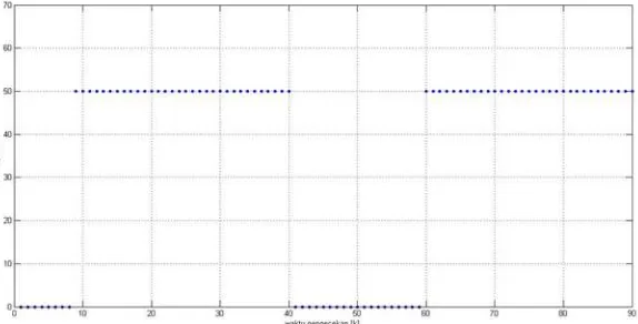
We given the maximum warehouse capacity (y_d) is 321 unit mass and can meet consumer demand for 50 unit mass everyday. The number of ordering in initial time is 204.6 unit mass. Figure 1 presented consumer demand for 90 days.

Figure 1. Consumer demand d kT

 

during k_{Numerical simulation} [image:8.595.169.456.235.381.2]

with MATLAB 7.6.0 (R2008a) obtained as follows

[image:8.595.170.456.427.574.2]

(9)

[image:9.595.151.508.78.269.2]

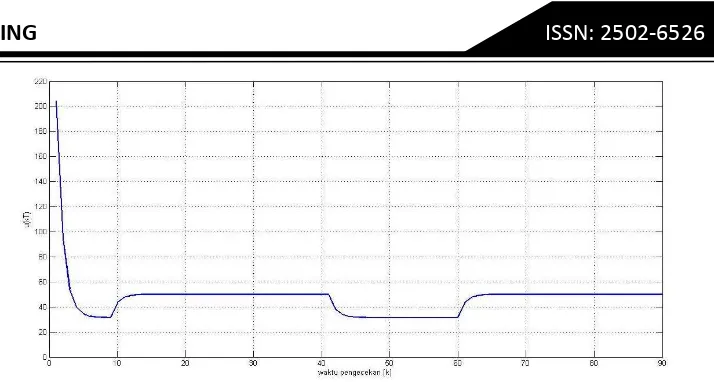
Figure 3. The number of ordering u kT

 

during k

The number of ordering u kT

 

is controler for the inventory system. It

must control the goods in warehouse not exceed the capacity but should still be able to meet consumer demand. Figure 3 shows about them, it will increase and decrease in line with fluctuations in demand.

If we want to change the parameters, then the number of goods in warehouse will not exceed the maximum capcity of the warehouse but should still be able to meet consumer demand, because it was guaranteed by Theorem 2 and Theorem 3.

4. CONCLUSION

The inventory system with linear quadratic regulator can optimize the number of ordering, despite the perishable goods. So, It will ensure that consumer demand will always be met , but not exceed the warehouse capacity. This controller is very useful if we have a perishable goods like radioisotope Luthesium-177 with half life 6.71 days, because the controller still work well to optimize them.

5. REFERENCES

Ignaciuk, P, and Bartoszewicz, A. (2010). Linear-Quadratic Optimal Control Strategy for Periodic-Review Inventory Systems. Automatica 46. pp. 1982-1993.

Ignaciuk, P, and Bartoszewicz, A. (2012). Linear-Quadratic Optimal Control of Periodic-Review Perishable Inventory Systems. IEEE Transaction on Control Systems Technology Vol.20, 1400-1407

Mital, K.V. (1976). Optimization Methods in Operations Research and Systems Analysis. New Delhi : Wiley Eastern Limited

(10)

Munawwaroh, Dita Anies, dan Sutrisno. (2014). Kendali LQR Diskrit untuk Sistem Transmisi Data dengan Sistem Jaringan Tunggal. Semarang : Jurnal Matematika Vol. 17 No.3. FSM UNDIP

Munawwaroh, Dita Anies. (2016). Aplikasi Kendali LQR Diskrit untuk Sistem Pergudangan Barang Susut dengan Peninjauan Berkala pada radioaktif I-131. Seminar Nasional Matematika dan Perndidikan Matematika. FPMIPATI - Universitas PGRI Semarang.. Semarang, 13 Agustus 2016

Ogata,K. (1995). Discrete Time Control Systems. Prentice-Hall

Olsder, G.J. (1994). Mathematical Systems Theory. The Netherlands : Delft Suyatno, Ferry. (2010). Aplikasi Radiasi dan Radioisotop dalam Bidang

Kedokteran. Dipresentasikan dalam Seminar Nasional VI SDM Teknologi Nuklir, Yogyakarta, 18 November 2010.