Land use discrimination based on textural characteristics

LAND

USE DISCRIMINATION

BASED ON

f

EXTURAL CHAWCTERISTICS

Bambang

Hendro Trisasongko

GRADUATE PROGRAM

BOGOR AGRICULTURAL UNIVERSITY

BOGOR

'

IQW'

"

Simple

but has extremely

deep

means

Kat

u

r:

Ibu'

,

Bapak

PREFACE

Environmental remote sensing is the measurement of earth featums from a distance. Many sensors have been built to identify, monitor and model the environmental condition. One of the largest applications of remote sensing is to i d e n t i land use. Land use data is overwhelmingly distributed and utilized by wide spread of users. In soil science domain, land use datais-used-in-pa~cutar for land evaluation or land management. Unknown or worst land use data

prevent further sustainable land uses or inhibit government policy in managing their land.

Analysis of remote sensing imageries was currently dominated by tone analysis as it is supported by wide range of image analysis softwares. However, latest trend on remote sensor technology, which produces higher spatial retsolution, reveals many aspect of interpretation, not only tonal data. New technology contained in SPOT, Landsat ETM+, IKONOS or Quickbid allow users

AUTHORS DECLARATION

I hereby declare that 1 am the

sole

author of the thesis titled "LAND USE DISCRIMINATION BASED ON TEXTURAL CHARACTERISTICS"

LAND

USE DISCRIMINATION

BASED ON

TEXTURAL CHARACTERISTICS

Bambang Hendro Trisasongko 99831 08

Thesis

as

a partial fulfillment leading to the degree of Master of Science in Soil Sciences

GRADUATE PROGRAM

BOGOR AGRICULTURAL UNIVERSITY

BOGOR

APPROVAL

Title : Land Use Discrimination based on Textural Characteristics Authsp : Barnbang Henelre Trisasengks

9983108 1 TNH Study Program: Soil Sciences

Approved

Board of Supervisors :

Dr. Boedi Tiahiono Chair

Dr.

M.

Nur Aidi

Member

Study Program of Soil Science

Head,

/c- L ~ L

Prof. Dr. Ir. Sudarsono, MSc _{nuwata, MSc}

BIOGRAPHY

Bambang Hsndro Trisassngko was born on 3 September 1970 in Batu, Malang.

He completed Elementary School and Junior High School in Turen, Malang.

Senior High School diploma was obtained in Malang. In 1988, he continued his undergraduate study at Bogor Agricultural University and took study program of

Soil Sciences with minor in Remote Sensing under guidance of Ir. Mahmud Arifin

Raimadoya, MSc and Ir. Tatat Sutarman Abdullah. Undergraduate thesis with

focus on development inpuvoutput program for image analysis was defended in

September 1993.

In 2000, he pursued graduate program on Soil ScienceILand Evaluation in Bogor

Agricultural University. For the thesis, he studied textural analysis applied on

aerial photograph, which may be replicated into another panchromatic systems such as radar or panchromatic channel of multispectral images. In graduate

program, he was supervised by Dr. Boedi Tjahjono and Dr. M. Nur Aidi.

He and his wife, Dyah Retno Panuju were gifted a daughter, Annisa Palupi in

ACKNOWLEDGEMENTS

Finally,

I

did.

First and most, I thank Allah SWT for allowing me alive and get many experiences in this world. Plenty

"rahmats"

have been given makes me easier to complete the thesis.

I owe a great deal to Dr. Boedi Tjahjono who sewed as chair

of

the board

of supervisor and teach anything I do not know in the field. Terima kasih Pak

Boedi.

Dr. Nur Aidi as member of the committee made significant contribution to many aspects in the thesis, particularly in statistics. Thank you for patience and constant question: "mana tesisnya dik Barnbang ?'. Terirna kccsih Pak Nur.

Author acknowledges and appreciates financial support provided by Dr. US Wiradisastra. He also help in many ways supporting my study in Soil Science.

Terima kasih

PC&

Uup.

Sewrral persons have a g m t deal suppart both financial and moral. I thank my former adviser (actually is still), Pak Mahrnud Raimadoya for being a father and friend in the same time. He is responsible for introducing me to the

fascinating world of radar and image analysis. Terima kasih Pak Mahmud. Staffs of Remote Sensing Lab. (Dr. Komama Gandasasmita, Dr. Ardiansywh, Dr. Baba Barus and Khursatul Munibah, MSc) create an exceUent academic atmosphere. Big thanks due to my colleagues in lab Diar "Dicky" Shiddiq and Manijo. Warm help from friends in LAPAN, particularly Bu Ita, Pak Santo and Pak Sudan is acknowledged.

Uncountable supports haves been provided by my family both in Turen, Malang and Ngadiluwih, Kediri. Thank you Pipit, for any help both in lab or home. I acknowledge help from Dr. Kardiyo Praptokardiyo's family since I stayed in Bogor. Thank you all, may God bless on you.

TABLE

OF CONTENTS

Preface

Acknowledgements

Chapter I

.

Introduction

...

Aerial Photograph

...

...

Digital Image. Tone and Texture

...

Objectives

Chapter 2

.

Common Practices in Image Analysis

...

Overview on Textural Transformation

...

Grey-Tone Spatial Dependence Matrix (GTSDM)

...

Remarks

on

Co-Occurrence Matrix Techniques

...

Classification Techniques: Unsupervised Approach

...

Assessing the Accuracy

...

Chapbr 3

.

Simple Statistical Texture Classification (SSTC)

...

Descriptive Measures of Distributions for Texture Measurement

...

....

ClassificationlSegmentatian Using Non-parametric Classification

...

Accuracy Assessment

Chapter 4

.

Rules of the Investigation

...

Sites

...

Methods

...

Chapter 5

.

Discussion

...

Sampling Technique. Preprocessing and Basic Statistics

...

Texture Characterization by Using Basic Statistical Elements

...

Class Separability Performance between Operators

...

...

Texture Transformation and Classification

Accuracy Assessment based on Field Observation

...

Chapter 6

.

Concluding Remarks

...

Conclusions

...

Suggestions

...

...

...

[image:76.566.85.472.162.482.2]

llST

OF FIGURES

Figure 1

.

Central pixel and its neighborhood

...

Figure 2

.

Orientation on Haralick's method

...

Figure 3

.

Sequential clustering processes ... Figure 4 . Iterative processing in ISODATA clustering ... Figure 5

.

Mathematical representation of error matrix ... Figure 6

.

.Convolution process ...p-...-.---...-.-A

-.

..

...

Figure 7

.

Box classifier decision boundaries in 2-d feature spaces

...

Figure 8

.

Modified box classification (MBC) decision boundaries

Figure 9 . Research sites

...

Figure 10

.

Research framework

...

Figure 11 . Sub-images on the sites

...

Figure 12

.

MEA performance on hypothetical image

...

Figure 13

.

Texture Transformation on Site I

...

Figure 14

.

Texture Transformation on Site 2

...

Figure 15 . Texture Classification on Site 1

...

Figure 16

.

Texture Classification on Site 2

...

LIST

OF TABLES

Table 1

.

Statistical properties of data

...

25 Table 2

.

Class discrimination by using minimum-maximum values in MBC

27

...

Table 3

.

Separability analysis on tea vs

.

forest in site I 28

Table 4

.

Separability analysis in site 2

...

29

...

Table 5 . Thresholding in site I 33

Table 6 . Thresholding in site 2

...

34

Table 7

.

Omission-commission matrices in site 1

...

38

Table 8

.

Omission-commission matrices in site 2

...

39

Table 9

.

Overall accuracy of site 1

...

40

Chapter

i

INTRODUCTION

Remote Sensing is defined as the technique of obtaining information about objects through the analysis of data collected by special instruments that are not in physical contact with the objects of investi~atjan (Av@ry and Berlin, 1992). As such, remote sensing can

be

-regard&- as --ffo#r a distance, Remate sensing thus dift'en

from

in situ sensing, where the instruments are immersed in, or physically touches the objects of measurement, such as portable

soil pH-meter.

In this decade, many remote sensing sensors have been developed for civilian applications, particularly for earth monitoring. In the early years of remote sensing development, peopllEtlscientists were using aerial photogmph to mr?duct

monitoring. In the further development, electromagnetic devictss were used instead of using photographic sensors,

In Indonesia, both systems are widely implemented. For instance, forestry sector still uses aerial photograph, while also uses landsat TM or SPOT data. The data are used in different applications. Aerial photograph is utilized to collect base informations such as topography, timber mluncz

pterdictjen,

etc In the

other hand, Landsat TM or SPOT are used for annual monitoring.

Aerial

Photograph

accuracy of the interpretation fully depends on the quality of photography and the analyst experience.

Photographic systems acquire spectral information with films of various spectral sensitivities. In order to maximize photo-interpretation result, it is important to select a film type, which will provide maximum contrast between dierent plant communities. Choices available for camera systems are color, color infrared (CIR) and panchromatic (black and white) films. First and widely implemented in Indonesia is panchromatic film.

Most aerial photograph analyst in Indonesia is still using manual interpretation technique. The technique has disadvantage since human ability is a major factor in analysis. This disadvantage may leads to inconsistency and inaccurate result, depends on experience of the analyst.

Recent development in computer and computing creates breakthrough in utilization of aerial photographs. In this decade, digital photogrammetry was widely introduced and followed by the industries creating tools for analysis. However, these tools mostly developed for specific utilizations such as topographic dsrlvation, utility mapping such as parcels, telecommunications, electricities, etc. Development of digital photogrammetry or interpretation for natural resources were less. The use of single or limited bandlchannel and no standard procedure in aerial photograph processing inhibits further development in natural resources applications. This research focuses on utilkatiin of digitized aerial photograph for land use discrimination.

Digital Image, Tone

and

Texture

Digital image as a pictorial information is represented as a function of two variables ( x , ~ ) . The image is stored in storage media as a two-dimensional array. If LX = {1,2, ... ,Nx) and Ly = {1,2, ... , Ny] are the X and Y spatial domains, then Lx x Ly is the set of resolution cells and the digital image I is a function which assigns

some gray-tone value G E fl,2, ... ,Ng] to each and every resolution cell; I:

Lx

x Ly ir G. Various two-dimensional analyses

are

performed on I to achieve specific image processing task

such

as

restoration, enhancement and classification.

entire agricultural field extending over a large number of resolution cells). The most difficult step in classification pictorial information from large block of resolution cells is that of defining a set of meaningful features to describe the pictorial information from the block (Haralick, st a/, 1973).

In search for meaningful features for describing pictorial information, Haralick ef al (1973) described three fundamental pattern elements used in human interpretation: spectral, textural and contextual. Spectral features describe the average tonal (grayscale) variation in various channsllband. Texture features contain information about distribution of grayscale variations

within specific channel. Contextual features contain information derived from blocks of pictorial data surrounding the area being analyzed. Context, tone and texture are always present in the image, although at times one feature may dominate others. In a small observation area, tone and texture dominate

interpretation process,

The notion of texture admits to no rigid description. Texture may be defined as "something composed of closely interwoven elements". The descrimon of interwoven elements is intimately tied to the idea of texture resolution, which one may think of as the average amount pixels for each discernible texture element. If this number is large, one can attempt to describe the individual elements in some detail. However, as this number near unity it becomes increasingly difficult to characterize these elements individually and they merge into less distinct spatial patterns (Ballard and Brown, 1982).

Jensen (1 996) provided another description of texture as follow. A discrete tonal feature is a connected set of pixels that all have the same or almost the

same gray shade (brightness value). When a small area of the image (e.g., a 3 x 3 area) has little variation of discrete tonal features, the dominant property of that area is a gray shade (tone). Conversely, when a small area has a wide variation of discrete tonal features, the dominant property of that area is texture.

Land use discriminations could be, done by using different approaches. In

framework was designed for manual interpretation. Since digital processing has different approach in interpretation scheme, adapting framework is necessary. However, some characteristics such as texture are challenging since it is exist in all natural imageries.

It is often found that classes of land coverlland use may be discriminated in digital imagery on the basis not only of their characteristic tone

(i.e.

mean digital number value) but also on their texture. Several authors have attempted qualitatively to define texture. Jensen (1996) notes that texture dominates when a small area has a wide variatin of discrete tonal features.

Several investigations on high-end image analysis softwares such as Erdas Imagine 8.3.1 and PC1 EasiPace 6.3 showed that texture dassifkation procedures are not

or

less supported. These sofhrvares basicalfy provide texture transformations only. Therefore the results of these processes are in

form

of texture imagers instead of texture-classified images. This condition is key factor in the research. Some proposed technique will be described in foilowing

chapters.

0

bjectives

The research has three primary goals:

Assess textural characteristics that derived from panchromatic images i.e.

aerial photograph

e Analyze textural transformation methodologies, particularly for land use

discrimination.

Chapter

ll

COMMON PRACTICES IN

lMAGE

ANALYSIS

Ovewiew on Textural Transformation

There is no rigid classification of textural analyses. Some authors used different classifications to describe developed techniques. Haralick et a/. (1 973) stated that early image texture studies have employed (i) autocorrelation functions, (ii) power spectra, (iii) restrided first-and second-order Markov meshes and (iv) relative frequencies of various gray levels on the unnomalized image. Meanwhile, Pratt (1991) described seven methods for analyzing texture features: (i) fourier spectra methods, (ii) edge detection methods, (iii) autocorreiation methods, (iv) decorrelation methods, (v) dependency matrix methods, (vi) microstructure methods and (vii) singular value decomposition methods. Detailed explanation is found on Haralick eta/. (1 973).

Let i = { I , 2, ... , Ni) represents configuration on horizontal s m a l domain, j

= { I , 2, ... , Nj) represents configuration on vertical spatial domain and k = { I , 2, ... ,

Nk) on spectral graylevel, then data arrangement could be described based on

spatial distance between central data (pixel) and its neighborhood. The arrangement then creates texture.

Figure 1. Central pixel and its neighborhood

We have seen that pixel e is acting as a central pixel. If spatial distance is assumed 1 (3 by 3 neighborhood), the neighboring pixel is constructed by pixels a, b, c, d, f, g, h and i. According to Ballard and Brown (1982), the 3 by 3 arrangement above is usually called Texel (Texture? Element). In order to describe smoothness of texture quantitatively, discrimination between arrangements (texels) was needed. Most statistical techniques develop their approach on texel discrimination.

Many researchers have developed texture analysis algorithms. However, there are no such standard methodologies for selection best approach. However, there is textural algorithm worth noted based only its wide implementation. The algoriihm is Grey-Tone Spatial-Dependence Matrix (Haralick, et a/., 1973).

Grey-Tone Spatial Dependence Matrix (GTSDM)

[image:83.566.74.473.49.772.2]

occurrences of pixel pairs of given greylevels at given displacement. Statistics like contrast, energy, entropy and so forth are then applied to the matrices to obtain texture features (Chen, 1995).

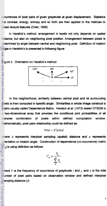
In Haralicks method, arrangement in texetls not only depends on spatial distance, but also on neighboring pixel position. Arrangement between pixels is determined by angle between central and neighboring pixel. Definition of rotation angle in Haralick's is presented in following figure.

Figure 2. Orientation on Haralick's method

In this neighborhood, similarity between central pixel and its surrounding pixels is then computed in specitic angle. Similarities in whole image construct a matrix usually called Dependence Matrix. Haralick et a!. (I 973) stated GTSDM is a two-dimensional array that provides the conditional joint probabilities of all paitwise combination of pixels within &fined computation window. Mathematically, pixel pairs relationship could be defined as:

where d represents interpixel sampling (6patial) distance and a represents orientation or rotation angle. Construction of dependence (co-occurrence) matrix

LCv] is using definition as follows:

[image:84.568.76.482.26.810.2]

Remarks on Co-Occurrence Matrix Techniques

Radiometric information plays an important role in remote sensing imageries. The radiometric information is represented by digital number or brightness value in a digital imagery. Recently, almost all algorithms applied on remote sensing image analysis are considering radiometric data collected by sensor as main data. Thematic extraction techniques such as classification employ digital number in their algorithms. Most multispectral imageries use 8-bit brightness scale, white other remote sensing platforms such as radar use 16 or 32 bit.

Since brightness value is relatively deep, computation time and size of occurrence matrix are important. For instance, if user use Landsat TM image with 8-bit depth or 256 greyscales, the algorithm will produce matrix as big as 256 by 256. Application on highly detailed imagery such as Radarsat, which produces 16- or 32-bit data, implies on extremely high volume of occurrence matrix. Sixteen-bit data will produce 65,536 x 65,536 matrix. Thirty-two bit data will have square matrix of 4,294,967,296. The matrix size is one major obstacle

in texture image analysis.

Schowengerdt (1997) stated that to reduce the computation burden, it is common practice to reduce the DN quantization (by averaging over adjacent DNs) to some smaller value and to average the co-occurrence matrix for different spatial directions. This technique might be applied on some images, particularly used by common image processing applications such as industrial imaging. On these kinds of imageries, specifically defined individual tone is not practically considered

as

an object in a scene. Therefore, techniques that alter pixels usually used to enhance information extraction. On remote sensing imagery, these kind of processing should be carefully taken. Alteration of digital number may shifts information gathering or creates bias on image understanding. In remote sensing image analysis, changing DN value of pixels is one of major concerns. Image enhancement such as stretching may create misinterpretation in digital image classification. In the simpb word, greyscale manipulation (i.e. greyscale compression) such as technique described by Schowengerdt is rather impractical on remote sensing data.

no further researches to develop texture classification scheme based on the methods.

Classification Techniques: Unsupewised Approach

Unsupervised classification is also called clustering, because it is based on the natural groupings of pixels in image data when they are plotted in spectral space. Cluster uses all or many of the pixels for its analysis and has no regard for contiguity of the pixels that define each cluster. There are several

methodologies to perform clustering.

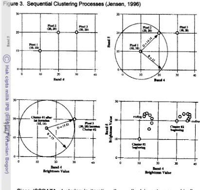
Most basic technique in clustering remote sensing image is Sequential Clustering. In sequential method, pixels are examined one at a time. The spectral distances between each analyzed pixel and the means of previously defined clusters are calculated. Each pixel either contributes to an existing cluster, or begins

a

new cluster, based on the spectral distances. Clusters are merged if too many are formed.

The sequential method requires little setup or preparation. There is only a few parameters need to be specified. The method usually performs faster than another approach such as ISODATA method. However, Sequential Clustering is slightly biased to the top of the image data. In the other word, this method is geographically biased and depends on location of first data being processed. ERDAS (1991) also reported that this method is parametric, meaning that the algorithm works on the assumption that the data distribution is normal.

[image:87.562.68.484.25.810.2] [image:87.562.71.482.88.478.2]

Figure 3. Sequential Clustering Processes (Jensen, 1996)

0 10 30 _{4 0}

Bvml4

Wlnras Value

Since ISODATA clustering is iterative, the method is not geographically biased to first location being processed. ERDAS (1 991) also noted that ISODATA is not as parametric as the other clustering methods and produce good

results for data that are not normally distributed. The main disadvantage of ISODATA is slow performance due to its multiiiterative processes.

Figure 4. Iterative processing in ISODATA clustering (ERDAS, 4991)

!SOU&" A, ',?st :';is$ ,c--r~,.- %&,-,.,- -:.-

' " , -2.:

!S(;,>AT.4 Ainioary i3iui:ter'j CIIMV' CU:UIMI rlew meens and etvd;,'?

'

:a l ~ t : l f r ~ a ~ ,-!l:si+( milan% In two-i:lmerlslorai Toc>clrlml 5r:aar

f

.I,, tr ₈ ! ₂ ... ... _{, a}

*

:

" n +

.,

;

L

Band A f i ~ l i d A

Assessing the Accuracy

Accuracy assessment determines the quality of the information derived from remote sensing imagery. Accuracy assessment can be qualitative or quantitative. The purpose of quantitative accuracy assessment is the identification and measurement of errors in the classified image. Quantitative assessment involves comparison between classified image and reference data. The reference data itself is assumed to be correct.

Congalton and Green (1999) stated that all accuracy assessment include four fundamental steps: (i) designing the sample; (ii) collecting data for each sample; (iii) building and testing the error matrix; and (iv) analyzing the resutts. Each step must be rigorously planned and implemented. Effective accuracy assessment requires (I) design and implementation of unbiased sampling

procedures, (2) consistent and accurate collection of sample data, and (3) rigorous comparative analysis of the sample data.

An error matrix compares information from reference sites to information derived from remote sensing data. The matrix is a square array of numbers set out in rows and columns that represent the labels of land use class assigned to particular category in one classification relative to the label of land use class assigned to particular category in another dassification. One of the classifications, usually the columns, is assumed to be correct and is called reference data. The another classification situated in rows is used to display classified labels derived from remote sensing data.

The error matrix can be considered effectiie way to represent accuracy due to its capability to describe both error of inclusion (commission emr) or error of exclusion (omission error). A commission error is defined as including an area into a category when it does not belong to that category. An omission error is

excluding that area from the category in which it truly does belong. Every error is an omission from the correct category a commission to a wrong category (Congalton and Green, 1999). In addition, the error matrix can compute another accuracy measures i.e. overall accuracy, producer's accuracy and user's accuracy. Mathematical representation of error matrix is presented in following figure.

Let assume that n pixels are distributed into k2 array where each sample

to one of the same k categories in the reference dataset (columns). Let n,

denote the number of pixels classified into category i where i = 1, 2, ... , k in

[image:89.570.77.463.20.816.2]

remote sensing image and category j where j = 1, 2, ..., k which represents reference data.

Figure 5. Mathematical representation of error matrix (Congalton and Green, 1999).

-

j = columns = refemnce row total

I 2 . . . k ni+

1 n1+

i = = _{2 n2+}

classification

. . . . . .

k nk+

column total n+j n+ 1 n+2 . . . n+k n

Number of pixel that classif'ied into category i in the remotely sensed classification is formulated as (Congalton and Green, 1999):

and number of pixels classified into category j in reference data is denoted as:

Chapter Ill

SIMPLE STATISTICAL TEXTURE CLASSIFICATION (SSTC)

There are two steps used to classify image based on textural information. First step is employing texture measurement, which transform original image into textured image. The second is classification or segmentation procedure that provides textu re-classified image.

Schowengerdt (1997) proposes method to reduce computation on co- occurrence matrix that is averaging over adjacent digital number. On non-remote sensing data, the technique may be considered. On the other hand, rernote- sensing imagery contains specific data in the pixel. Therefore retaining data is one of major concern in digital image analysis. Objection on Schowengerdt's statement is main direction in this research. This objection showed importance to pursue a comprehensive experiment starting with basic statistics. A simple basic statistics framework will be designed by employing descriptive measures of distributions.

Local statistic methods could be used as starting point to assess existence of textural information, Computation of statistical measurement is practically same with technique usually used for assess basic statistic of an image. The only difference is applied data. Basic statistic computation is usually applied on whole digital number with smallest unit of observation is a pixel. Later, we! will discuss on texel as smallest unit of observation.

Descriptive Measures of Distributions for Texture Measurement

There are two kind of measures usually used to describe distribution function of data: (i) measures of centrality; and (ii) measures of variability (Barnes, 1994). Measures of centrality refer to the location or centrality of a probability distribution function and consist of three theoretical quantities i.e.

p = xp(x) for discrete distributions

p =

J

xf (x)& for continuous distributions

Mean is the most commonly used average of a distribution and can be obtained readily with data processing. However, another measure could be used also for measuring central tendency. Median is defined as the middle value when data are arranged in an array according to size (Longley-Cook, 1970).

Another useful measure of the center tendency is the mode. When there are a number of values at each point or in each class, the point or class with the greatest number is called the mode. When a frequency curve has been drawn, the mode is the maximum point on the graph. Occasionally there is no mode or more than one mode (Longley-Cook, 1970). This condition creates less useful implementation on this research since each texture needs to be characterized by its histogram.

Two separate sets of data may contain the same number of items and have the same mean but one set may be much more dispersed or spread about the average value than the other. A measure of dispersion or variation from the mean is needed to help define the distribution more fully.

Longley-Cook (1970) describes six types of measurement to assess dispersion.

I. The Range. The difference between the largest and the smallest values.

2. The 10-90 Percentile Range. The difference between the 1 0 ~ and 9oth

percentile points.

3. The Semi-lnterquartile Range or Quartile Deviation. One-half the difference between the first and third quartiles.

4. The Avenge Deviation from the Mean or Mean Devi9tion. This is the

arithmetic mean (average) of the individual absolute values of the deviations from the mean.

5. The Standard Deviation or its square, the Varience. This is mod generally

used measure of dispersion.

In this research, author used four statistical descriptors for characterizing land use texture i.e. Greyscale Range (RGE), Mean (MEA), Variance (VAR), and Entropy (ENT). Fitst three descriptors were adopted from Longley-Cook (1970). The last method was proposed as additional and comparative descriptors.

A distribution can be categorized by a single, information, measure called Entropy. This measure is the average uncertainty of the various proportions, and is calculated by the formula (Johnston and Semple, No Date):

where

pi is the proportion in the i-th component of the distribution n is the number of components in the distribution, and

H is the information measure (Entropy)

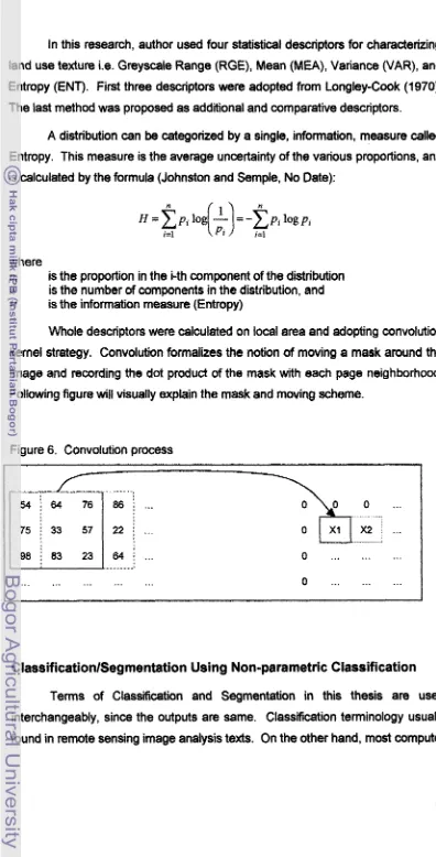
[image:92.568.74.470.50.828.2]

Whole descriptors were calculated on local area and adopting convolutibn kernel strategy. Convolution formalizes the notion of moving a mask around the image and recording the dot product of the mask with each page neighborhood. Following figure will visually explain the mask and moving scheme.

Figure 6. Convolution process

ClassificationlSegmentation Using Non-parametric Ciassification

vision books refers it as Segmentation. However, Classification and Segmentation have not perfectly same meaning.

Shapiro and Stockman (2001) stated that the term of image segmentation refers to the patiition of an image into a set of regions that cover it. The goal in many tasks is for the regions to represent meaningful areas of the image, such as crops, urban areas and forests of a remote sensing image.

Classification strategy is closely related to the amount of data, including its variable (in remote sensing image analysis means number of bands). Recently, many classification algorithms have been developed based on multivariate statistics or combined with another approach such as fuzzy or neural network. However, classification methodology for single band remote sensing data is less constructed.

Classification algorithms may be grouped into one of two types: parametric or non-parametric. Parametric algorithms assume a particular class statktical distribution, commonly the normal distribution, and require estimates of the distribution parameters, such as the mean vector and covariance matrix, for classification. Non-parametric algorithms make no assumptions about the probability distribution and are often considered robust because they may work well for a wide variety of class distfibutions, as long as the dass signatures are

reasonably distinct (Schowengerdt , 1 997).

Classification scheme in this research is built based on classification strategy developed in radar image processing. This is due to similariiy condition between single polarization radar and digital airphoto, i.e. single band data. Several authors have developed some single-band classification approaches. First and widely utilized approach is by implementing threshdding technique. Second approach is based on spatial similarity and usually called region growing. Third approach is employing edge detection mechanisms.

There are two main steps in classification by thresholding. First step is to assign a class label to each pixel according to its intensity value:

IN

f I (x , y ) 6

Emin, max]

class(x, y ) =

Then, pixel-labeling algoriihm is used to assign the same label to the connected pixels belonging to the same class. The pixels, which have the same label, are connected and form part of a single segment (Beaulieu and Najeh, 1997).

Region growing algoriihm requires two parameters to initiate segmentation i.e. a window size and a threshold. A window is associated to each seeded pixel where initial values are estimated. It is assumed that an optimum size window exists that differentiates the most the values related to each seeded pixel windows. To decide if a pixel is aggregated to a region, a difference between tested pixel window and the initial one is obtained; if this value does not exceed a certain threshold, the tested pixel is incorporated into the region (Lira et

a/., 1996). Authors including Shimabukro et al. (1997) and Costa et al. (1997)

have reported some successful

works.

However authors notice about difficulties and subjectivity on initializing seed region.

Third approach basically uses edge detection algorithms such as Sobel, Laplacian or higher technique such as Mough transform. This approach was less implemented since the algorithm only provides boundary for different class and does not provide "label" for each class.

This research only focus on thresholding technique due to its computationally effiient and reliable for basic discrimination between groups of data. Based on this technique, author proposes Modifled Box Classifier (MBC). Modified box classifier is developed based on Box Classifier with only one feature space. Schowengerdt (1997) state that Box classifier is perhaps the simplest of all classification methods. A set of k-dimensional boxes, centered at estimated classes mean vectors, are placed in k-dimensional feature space. If an unlabeled pixel vector lies within one of the boxes, it is assigned that class label. Decision boundaries are set by vectors of means and standard deviations.

Modification should be done to allow digital aerial photograph to be processed. Simple modification is applied here by using only one dimension feature space. One dimension feature space of Figure 7 is presented in Figure 8.

[image:95.566.73.455.39.787.2] [image:95.566.77.378.50.503.2]

Figure 7. Box classifier decision boundaries in

2-6

feature spaces

Figure 8. Modified box classification (MBC) decision boundaries.

DN2 ... ? _... i . . ; { i

; i j

i

Class A f

i

Class B

j

. _{. ...}

i i ! + DNl

... .)

I

... ...,

i j

j Class A

i

...

i i

. . j

: :

... :

j

Class B

1

... ,

b

Accuracy

Assessment

DNI

C

In this research, proposed accuracy assessment is following error matrix technique as described by Congalton and Green (1 999). l-fowever, modification will be applied in order to fit the cumnt condition. In their book, Congalton and Green (1999) used sampling technique to collect brightness value data. This sampling data will be used to compute error matrix. Instead of using sampling

Chapter

lV

RULES

OF

THE

INVESTIGATION

In this research, some tools are utilized i.s. computer with remote sensing software and Microsoft Visual Basic 5 Control Creation Edition compiler. Another device is HP ScanJet 6100 Scanner System. In fieldwork adivrty, author utilize one unit of Global Positioning System Gamin 12XL (including downloader unit) and a portable computer (notebook).

Sites

In this research, author used two locations in Cianjur Regency for analysis based on aerial photograph data. First location was in Pacet and relied on south- east slope of Mt. Gede-Pangrango. Second location was east slope of same mountains in area of Punwk. First image in Pacet consists of two land use classes i.e. forest and tea. Second image in Puncak has three land use dames: (i) forest; (ii) mixed garden and (iii) bare phase of paddy field, Figure 9 shows the original images.

Methods

[image:97.566.78.471.75.574.2]

Figure 9. Research Sites

Site 1

(Pacet) Forest

Tea

Site 2

(Puncak) _Forest

PaddvIBare Land

Mixed Garden

Good-conditioned and geocorrected aerial photographs are selected and scanned in 150 dpi. The use of higher resolution may be applied. However, higher resolution significantly increases data and in particular resolution, no information gained further. Selection of land usg class is then performed. First test of Simple Statistical Texture Classification (SSTC) will be applied on imagette with simple class discrimination. Another test is the apptied on more complex imagettes.

convolution window. Relationship between distance lag

(4

and convolution window (w) is defined as

In this research, author used 4 types of convolution windows that are 3x3, 5x5,

7x7, and 9x9. The use of 3x3 window usually produces crisp output but less generalized polygon.

Fieldwork is intended to map selected areas. Usually, field check is done in only one or mote locations related to its class. This approach has limitation since actual boundary is not particularly defined. Usually samples are taken far from the boundary. In order to minimize bias on boundary areas, author use field mapping method. However, since mapping is done in the field, this method

needs intensive work on the field. Fieldwork will utilize Garmin GPS to derive land use boundaries. Since GPS system limits obsentation points to 500 nodes, a portable computer (laptop or notebook) and GPS downloader unit are required.

This step produced a reference map.

Gaoometitad

/

Photograph

/

t

1

Scanning on 150 dpi

1

L--T----

L.,

I X n d wlectim 1

-

7

I

3

-- TextureAnalj%is

7

with diffarant lag

L-

--

A

4-

I

Field work and

/ Texture Characterization 1

1

and Classification

1

L-v-

Reference Map

i i

\ Field-baasd 1

1

Accuracy Assemment

I

Chapter V

DISCUSSIONS

Sampling Technique, Preprocessing

and

Basic Statistics

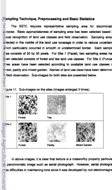
[image:100.566.71.464.141.807.2]

The SSTC requires representative sampling area for discrimination purpose. Basic appropriateness of sampling area has been selected based on visual recognition of land use classes and field obsetvation. Sampling area is selected in the middle of the land use coverage in order to reduce uncertainty, which particularly occurred in smooth or undetermined border. Each sampling area consists of 30 by 30 pixels. For Site 1 (Pacet), two sampling areas have been selected consists of forest and tea land use classes. For Site 2 (Puncak), three areas have been selected according to available land

use

classes i.e. forest, paddy and mixed garden. Names of land use class have been determined in field observation. Sub-images for both sites are presented below.

Figure 11. Sub-images on the sites (images enlarged 3 times).

Forest Tea

I

1

1

Forest Paddy Mixed Garden

sensor and developed by chemical reactions. Photograph appearance is strongly determined by time of photographic processing. Aerial photograph also has poor radiometric calibration and validation, which usually used to maintain image quality products. A fact that forests in Site 1 and Site 2 are visually dierent particularly for tonal arrangement is basically determined by unbalanced quality product. By using satellite images, the weaknesses may be avoided.

This research is intended to characterize texture in different condition. In this research, conditional aspect is only determined by spatial distance (lag) between central pixel and its neighborhood in a convolution kernel. The research uses 4 types of lag, i.e, 1 (or 3x3 kernel), 2 (or 5x5 kernel), 3 (or 7x7 kernel) and 4 (9x9 kernel). The lags can be used to assess sensitivity in texture discrimination.

Preliminary processing for basic statistical computation is required for describing the data. In this research, basic statistical computation involves search for minimum and maximum value, and calculating mean and standard deviation. Result is described in Table ?.

Texture Characterization by

Using

Basic Statistical

Elements

In this research, texture characterization is derived from analogy of box classification as described in Chapter Ill. Standard box dassifier uses two or more feature space to describe each class on the image. Since this research used panchromatic image, modification of standard box classifier is proposed. In this time, the modification is simply called Modified Box Classifier (MBC).

The MBC requires basic statistical information based on sample images that describe textural information of each land use. Those basic informations are mean and standard deviation. Textural information was then derived by characterizing each mean and standard deviation on each class. With those statistical informations, boundary (minimum and maximum values) of each land use class may be calculated. Minimum

and

maximum values of MBC follow basic specification of Box Classifier as described below:

Table 1. Statistical properties of data

Site I. Pecet

Tea Forest

I

Min Max Mean SD Min Max Mean SD

11 31.00 105.00 70.92 19.45 179.00 233.00 208.10 12.42

Site 2. Puncak

Forest paddy M iGarden

I

Min Max Mean SD Min Max Mean SD Wn Max Mean

11 100.00 161.00 135.20 12.43 59.00 136.00 90.68 14.93 61.00 146.00 102.11

13 22.00 125.00 74.82 21.19 3.00 107.00 42.99 18.1 1 9.00 128.00 53.40 14 104.56 197.44 155.03 19.10 164.00 247.89 200.89 20.63 111,11 199.89 154.52 15 51.21 1790.40 608.70 326.30 0.77 1385.51 226.65 193.84 12.91 1498.67 300.76 16 1.68 2.20 2.14 0.09 0.94 2.20 2.06 0.18 1.52 220 2.10

Note:

Image # I : RGE Operator with lag 4 Image t 9 : RGE Operator with lag 2

Image #2 : MEA Operator with lag 4 Image #I 0 : MEA Operator with lag 2

Image #3 : VAR Operator with lag 4 Image # I 1 : VAR Operator with lag 2

Image #4 : ENT Operator with lag 4 Image # I 2 : ENT Operator with lag 2

Image #5 : RGE Operator with lag 3 Image #I3 : RGE Operator with lag 1

Image #8 : MEA Operator with lag 3 Image #I4 : MEA Operator with lag 1

Image #7 : VAR Operator with lag 3 Image #I5 : VAR Operator with lag 1

Image #8 : ENT Operator with lag 3 Image kt16 : ENT Operator with lag I

Wih the minimum-maximum values, class separation analysis is possible to be evaluated. This information is important to characterize discrimination

between textural information of available land use classes. Class separation analysis is implemented by using all minimum-maximum values, which plotted into a feature space. If class overlap is none or minimum, class discrimination may be considered as good. Class discrimination between two sites is presented in Table 2.

Class

Separability Performance

between Operators

In this section, performance of operators will be assessed. Evaluation may be based on (i) class versus class assessment; or (ii) aggregate assessment. First method proposed is used for detailed examination of operator performance. This method is useful for learning texture pattern of specific land use class and its difference with another land use classes based on sampling sites. The second is used for evaluation of operator performance in aggregate and involving whole image. Information contained can be used for predicting accuracy for whole imagery.

In Site 1 (Pacet), almost all operators have good performance in separating between Tea and Forest, except MEA operator. This phenomenon can be understood since mean operator is highly affected by extreme high and low frequencies in brightness value. If the tone is quite similar such can be seen in Tea area, MEA operator may be utilized. However, this operator is less sensitive to discriminate land use class with coarse texture such as forest or growth

estates. Details on separability analysis on Site 1 is presented in Table 3.

Table 2. Class discrimination by using minimum-maximum values in MBC.

Site I, Pacet

Image Tea Forest

.#

I

Min Max Min Max

11 51.47 90.38 195.68 220.52

Image Forest paddy Mixed Garden

#

I

Min Max

1

Min Max

1

Min Max

1 122.77 147.631 75.75 105.611 80.95 123.27

Note:

lmage #l : RGE Operator with lag 4

lrnage #2 : MEA Operator with lag 4

Image #3 : VAR Operator with lag 4 Image #4 : ENT Operator with lag 4

lrnage #5 : RGE Operator with lag 3

lmage #6 : MEA Operator with lag 3

lmage #7 : VAR Operator with lag 3

lmage #8 : ENT Operator with lag 3

Details on operator were described on Chapter Ill.

lmage #9

lmage #I0 lmage # I 1 Image #I2 lmage #I3 Image # I 4 lmage # I 5

lmage #I6

: ROE Operator with lag 2 : MEA Operator with lag 2

: VAR Operator with leg 2 : ENT Operator with lag 2

: RGE Operator with lag I

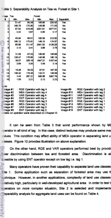
Table 3. Separability Analysis on Tea vs. Forest in Site 1.

Image Tea Forest

#

I

Min Max

I

MSn M a

I

Separable

11 51.47 90.381 195.68 220.521 Yes

2 3 4 5 6 7 8

160.79 175.00 87.52 318.09

3.33 3.67

9

10 11 12

Note:

lmage # I : RGE Operator with lag 4

lmage #2 : M€A Operator with lag 4

Image #3 : VAR Operator with lag 4

lmage #4 : ENT Operator with lag 4

lmage W : RGE Operator with lag 3

lmage #6 : MEA Operator with lag 3

lmage #7 : VAR Operator with lag 3

lmage #8 : ENT Operator with lag 3

Details on operator wen? described on Chapter Ill.

40.94 80.01 160.12 175.91 65.56 311.47 3.1 0 3.41

13 14 15 16

lmage #Q : RGE Opemtor with lag 2

Image #I0 : MEA Operator with lag 2

Image #11 : VAR Operator with tag 2

Image #I2 : ENT Operator with lag 2

lmage #I 3 : RGE Operator with lag 1

Image # I 4 : MEA Operator with lag 1

Image # I 5 : VAR Operator with lq 1

Image #I6 : ENT Operator with lag 1

149.06 171.55 2251.61 3077.91

4.06 4.17

31.09 67.22 159.47 176.85 38.07 305.16

2.69 3.00

It can be seen from Table 3 that worst performance shown by MEA operator in all kind of lag. In this case, distinct textures may produce same mean values. This condition may affect ability of MEA operator in separating land use classes. Figure 12 provides illustration on above explanation.

No Yes

Yes

182.59 212.82 148.10 174.87 2041.52 3136.28

386 3.78

19.28 5023

158.42 178.45 3.45 287.21

1.89 2.21

On the other hand, RGE and VAR operators performed best by providing clear discrimination between tea and forested area. Discrimination is also possible by using ENT operator except on low lag i.e. lag 1.

Yes No Yes Yes

156.85 199.68 140.96 180.19

1647.21 3167.44

3.08 3.19

Many operators have proven their capability to separate land use classes in Site 1. Some application such as separation of forested area may use this technique. However, in another applications, complexity of land use classes is relatively high, particularly in well-developed agricultural area. In order to test the operators on more complex situation, Site 2 is selected and implemented. Separability analysis for aggregate land uses can be found on Table 4.

Yes No Yes Yes

97.61 167.30 132.21 189.09 890.86 3007.76

2.12 223

Yes No Yes

[image:105.566.77.466.58.823.2]

[image:106.566.70.459.67.818.2]

Figure 12. MEA performance on hypothetical image I

Mean 111.11

Range 200

Mean 111.11

Range 2

Table 4. Separability Analysis in Site 2.

Note:

lmage # I : RGE Operator with lag 4

lmage #2 : M€A Operator with lag 4

lmage #3 : VAR Operator with lag 4

lmage #4 : ENT Operator with lag 4

lmage #5 : RGE Operator with lag 3

lmage #6 : MEA Operator with lag 3

lmage #7 : VAR Operator with lag 3

Image #8 : ENT Operator with lag 3

Details on operator were described on Chapter Ill.

lmage #9

lmage #I0

lmage #I 1

lmage #12

lmage # I 3 lmage #I4 lmage #I5 lmage #I6 Image # 1 2 3 4 5 6 7 8 9 10 11 12 13 14 15 16

: RGE Operator with lag 2

: MEA Operator with lag 2

: VAR Operator with lag 2

: ENT Operator with lag 2

: RGE Operator with lag 1

: MEA Operator with lag 1

: VAR Operator with lag I

: ENT Operator with lag 1

Forest

Min , Max 122.77 147.63 144.94 184.12 763.89 1052.98

3.90 4.01

107.86 138.19 143.74 165.61 689.02 1049.07

3.53 3.68

87.36 123.71 141.35 168.26 537.99 1060.35

2.98 3.14

53.63 96.01 135.93 174.14 280.40 933.00

2.05 2.23

1 Separable Yes No No No Yes No No No Yes No No No Yes No Yes No paddy

Min Max

75.75 105.61 189.60 212.65 292.91 758.07

3.66 3.90

65,42 95.26 187.09 215.00 233.33 668.60

3.30 3.60

49.02 82.81 184.11 217.85 136.61 582.99 2.75 3.1 1

24.88 61 . I 0 180.26 221.53 32.81 420.48

1.88 2.24

Mixed Garden

Min Max

80.95 123.27 146.33 162.70 338.93 591.97

3.71 3.89

71.45 112.46 145.12 164.35 292.68 591.38

3.40 3.58

58.67 96.36 143.01 i66.56 216.00 577.61

2.88 3.10

35.74 71.05 138.97 170.07 94.87 506.66

Site 2 is designated to re-evaluate findings on Site 1 with more complex

land use classes. Table 4 shows RGE operator has best performance in separating land use ctasses. The performance is quite similar to RGE performance in Site 1. A more complex situation has inhibits performance of both VAR and ENT. In Site 1, VAR has strong capability and similar to RGE's

performance. However, in Site 2, VAR can not separate land use classes particularly for paddy versus mixed garden. In many kind of lag, didmination between paddy and mixed garden can not be done statistically by VAR operator,

except lag 1.

Texture Transformation and Classification

Before classification procedure applied, the raw image should be transformed into ttaxtum data. This step involves texture transformation. Texture transformation is basically same technique with those applied on texture characterization. The main difference is image being

used.

Texture characterization is applied only on sub-image, which represents each land use

class.

On

the other hand, texture transformatiin is apptted

on

whole data bsmg

[image:108.562.51.468.87.545.2]

[image:109.566.75.472.92.534.2]

Figure 14. Texture Transformation on Site 2.

MEA

1

Operator

VAR ENT

Lag 3

Summarizing transformation results, there is close relationship between separability analysis and transformed images.

In

Site 1, separability analysis informed that MEA operator has failed to discriminate clearly on tea and forest. Result from transformation also showed unsuccessful differentiation between both land use classes visually. On the other hand, RGE, VAR, and EN7 operators have been successful, except ENT operator applied on lag 1. Even small distinction can be visually assessed in ENT 1, discrimination between land

use classes can not be separated statistically.

performance in both sites, RGE operator performs best and relatively constant in discriminating land use classes.

Separability analysis may be used to predict the classification. However, in order to quantify accuracy, classification procedure has been taken. From separability analysis, land use classes were almost separable in some images. This condition is occurred more on complex images such have been shown on %te 2 images. In order to focus on classification performance, operator that fail to separate defined classtm will be rejected in classification step. Threshold

boundaries on both sites are presented in Tabla 5 and 6.

Threshold boundaries are set by sorting minimum value of each land use class. Process is then followed by computing hatF-difference between maximum value of first-sorted land use class and minimum value of second-sorted class. This approach is major distinction to common Box Classifier, which allowing classifier to minimize unknown or unclassified pixels.

Table 5. Thresholding in Site I.

Note: lmage # I lmage #2 lmage #3

lmage #4

lmage #5

Image #6

lmage #7

Image #8

Image # 1 2 3 4 5 6 7 8 9 10 11 12 13 14 15 16

: RGE Operator with lag 4

: MEA Operator with lag 4 : VAR Operator with lag 4 : ENT Operator with lag 4

: RGE Operator with lag 3

: MEA Operator with lag 3

: VAR Operator with lag 3

: ENT Operator with lag 3

lmage #9 : RGE Operator with lag 2

lmage #I0 : MEA Operator with lag 2

lmage # I 1 : VAR Operator with lag 2

Image #I2 : ENT Operator with lag 2

Image #I3 : RGE Operator with lag 1

Image #I4 : MMEA Operator with lag 1

Image # I 5 : VAR Operator with lag 1

Image # I 6 : ENT p e t o r t h lag 1

Threshold 143.03 166.17 1284.85 3.86 131.30 167.49 1 176.49 3.54 112.04 168.16 976.18 3.04 73.92 168.44 589.04 2.1 7 Tea

Min Max

51.47 90.38 160.79 175.00 87.52 318.09 3.33 3.67

40.94 80.01 160.12 175.91

65.56 311.47 3.10 3.41

31.09 67.22 159.47 176.85

38.07 305.16 2.69 3.00

19.28 50.23 158.42 178.45

3.45 287.21 1.89 2.21

F meet

Min Max

195.68 220.52 149.06 171.55 2251.61 3077.91 4.06 4.17

182.59 212.82 146.10 174.87 2041.52 31363.28

3.66 3.78

156.85 199.68 140.96 180.19 1647.21 3167.44

3.08 3.19

97.61 167.30 132.21 189.09 890.86 3007.76 2.12 223

[image:110.566.73.462.50.801.2]

Table 6. Thresholding in Site 2.

Threshold computation is then followed by classification by using Modified Box Classifter (MBC). For Site 1, thmshold value will separate land use classes of tea and forested areas. Digital numbers that lie between minimum to threshold value will be set to tea class. On the other hand, numbers that greater than threshold is classified into forest.

For Site 2, two threshold have been set to determine boundary classes for three land use classes, i.e. forest, paddy and mixed garden. Pixel has digital number less than threshold 1 will be categorized into paddy. Greyscale values that fit between threshold I and threshold 2 will be classified into mixed garden and values greater than threshold 2 is set for forest.

Threshold2 123.02 110.16 91 $86 62.34 393.53

Resutts on texture classification for Site 1 and Site 2 are presented on Figure 15 and 16 respedively,

Image #I : RGE Operator with lag 4 Image #9 : RGE Operator with lag 2

Image 42 : MEA Operatar with lag 4 Image 410 : MEA Operator with lag 2

Image #3 : VAR Operator with lag 4 Image # I 1 : VAR Operator with lag 2

Image #4 : ENT Operator with lag 4 Image # I 2 : ENT Operator with lag 2

Image #5 : RGE Operator with lag 3 Image # I 3 : RGE Operator with lag 1

Image #6 : MEA Operator with lag 3 Image # I 4 : MEA Operator with lag 1

Image #7 : VAR Operator with lag 3 Image #I 5 : VAR Operator with lag 1

Image #8 : ENT Operator with lag 3 Image # I 6 : ENT Operator with lag 1

lmage # 1 2 3 4 5 6 7 8 9 10 I 12 13 14 15

! 6

Note:

Mxed Garden

Min Max

80.95 123.27 146.33 162.70 338.93 591.97

3.71 3.89

71.45 112.46 145.12 164.35 292.68 591.38

3.40 3.58

58.67 96.36 143.01 166.56 216.00 577.61

2.88 3.10

35.74 71.05 138.97 170.07 94.87 506.66

1.98 2.22

ores st

Min Max

122.77 147.63 144.94 164.12 763.89 1052.98

3.90 4.01

107.86 138.19 143.74 165.61 689.02 1049.07

3.53 3.68

87.36 123.71 141.35 168.26 537.99 1060.35

2.98 3.14

53.63 96.01 135.93 174.14 280.40 933.00

2.05 2.23

Sepmhle Yes No No No Yes No No No Yes No No No Yes No Yes No paddy

Min Max

75.75 105.61 189.60 212.65 292.91 758.07

3.66 3.90

65.42 95.26 187.09 216.00 233.33 668.60

3.30 3.60 <