i
RICE PRICE VOLATILITY, ITS DRIVING FACTORS AND
THE IMPACT OF CLIMATE CHANGE ON PADDY
PRODUCTION AND RICE PRICE IN INDONESIA
SILVIA SARI BUSNITA
POSTGRADUATE SCHOOL
BOGOR AGRICULTURAL UNIVERSITY BOGOR
STATEMENT LETTER OF THESIS AND SOURCE OF
INFORMATION
I declare that thesis entitled Rice Price Volatility, Its Driving Factors and The Impact of Climate Change on Paddy Production and Rice Price in Indonesia is my own work with guidance of the advisors and has not been submitted in any form at any college, except Bogor Agricultural University. The sources of information derived and quoted from published and unpublished works of other authors mentioned in the text are listed in the Bibliography at the end of this thesis.
Hereby I transfer the copyright of this thesis to Bogor Agricultural University.
SUMMARY
SILVIA SARI BUSNITA. Rice Price Volatility, Its Driving Factors and the Impact of Climate Change on Paddy Production and Rice Price in Indonesia. Supervised by RINA OKTAVIANI and TANTI NOVIANTI.
The issue of food security as the spillover effects of 2007-2008 global crisis resulted in a surge in food prices at the consumer level around the world. Rising food prices have become a burden for the poors in developing countries who spend on average half of their household income on food, especially on cereal commodities. Meanwhile, in the last decades, there have been an increase number of floods and periods of drought, devastating cyclones, water, soil and land resources that are continuing to decline in several parts of the world. The impact of these global climate change phonemonen could be seen as the production yield of main crops in tropical countries had become fluctuated. Thus, this has affected the food price fluctuations especially on the grain price both in international and domestic markets. The rice-commodity, who had been known for its thin market characteristics, also experiencing the fluctuation in production, its productivity and also the rice price. Considering the importance of rice as the main staple food in Indonesia, the purpose of this research is to identify the Indonesia rice price fluctuation (volatility), to investigate what are the main drivers that causing the fluctuation of local rice price in Indonesia; and the last one is to investigate the consequences of climate change variables (especially temperature changes) towards Indonesian paddy production, local rice price, and its fluctuation (volatility).
By applying monthly time-series data from 2007 to 2014, this research used ARCH-GARCH (Autoregressive Conditional Heteroscedasticity-Generalized Autoregressive Conditional Heteroscedasticity) methods to find out the rice price volatility. The results find that there exist the volatility (fluctuation) in Indonesian rice price variable and time varying, with the highest price spikes happened on 2010 and 2011 respectively. While using the VECM (Vector Error Correction Model), it shows that the driven factors affects the Indonesia local rice price fluctuation are paddy production, temperature changes, national domestic stock of rice, world rice price, household comsumption, exchange rate, and interest rates in the long-run. According to Impulse Response analysis result, the climate changes (the temperature changes), would affect negatively the paddy production in Indonesia both in the short run and long run. On contrary, the temperature changes would be positively influence the rice price and also its fluctuation in Indonesia. These results are important for the stakeholders and government to prevent the risk of paddy production uncertainty and rice price fluctuation caused by climate change in the future.
vi
RINGKASAN
SILVIA SARI BUSNITA. Volatilitas Harga Beras, Faktor Penyebab dan Pengaruh Perubahan Iklim terhadap Produksi Padi dan Volatilitas Harga Beras di Indonesia. Dibimbing oleh RINA OKTAVIANI dan TANTI NOVIANTI.
Isu keamanan pangan sebagai spillover effects dari krisis global tahun 2007-2008 lalu, salah satunya ditandai dengan lonjakan harga pangan di tingkat konsumen di seluruh dunia. Peningkatan harga pangan ini menjadi beban bagi masyarakat miskin di negara berkembang yang menghabiskan rata-rata setengah dari pendapatan rumah tangga mereka untuk pangan, terutama pada komoditas serealia (padi-padian). Sementara itu selama beberapa dekade terakhir telah terjadi peningkatan banjir, kekeringan, perubahan siklus hujan, maupun cuaca ekstrem di beberapa bagian dunia sebagai pertanda dari perubahan iklim global. Akibat dari fenomena ini hasil produksi tanaman pangan utama di negara-negara tropis menjadi berfluktuasi. Hal ini mempengaruhi fluktuasi harga makanan terutama pada harga pangan pokok baik di pasar internasional dan domestik. Beras sebagai salah satu komoditi pangan utama dengan karakteristik pasarnya yang “tipis” (jarang diperdagangkan), juga mengalami fluktuasi dari segi jumlah produksi, produktivitas maupun harga. Mengingat urgensi beras sebagai makanan pokok utama di Indonesia, tujuan dari penelitian ini adalah untuk mengidentifikasi fluktuasi (volatilitas) harga beras di Indonesia, menganalisis faktor pendorong utama yang menyebabkan fluktuasi harga beras di Indonesia; serta menganalisis pengaruh variabel perubahan iklim (terutama perubahan suhu) terhadap produksi padi, harga beras lokal dan fluktuasi (volatilitas) harga beras Indonesia.
Penelitian ini menggunakan data sekunder time-series bulanan dari tahun 2007 sampai 2014. Metode yang digunakan untuk menganalisis volatilitas harga beras adalah ARCH-GARCH (Autoregressive Conditional Heteroscedasticity-Generalized Autoregressive Conditional Heteroscedasticity). Hasil analisis volatilitas menunjukkan bahwa harga beras Indonesia merupakan variabel ekonomi yang bersifat volatile, time-varying (bervariasi antar waktu), dengan lonjakan harga tertinggi terjadi pada tahun 2010 dan 2011. Sementara berdasarkan hasil estimasi VECM (Vector Error Correction Model), menunjukkan bahwa faktor-faktor yang signifikan mempengaruhi fluktuasi harga beras Indonesia dalam jangka panjang adalah produksi padi, perubahan suhu, cadangan beras domestik nasional, harga beras dunia, jumlah konsumsi rumah tangga, nilai tukar, dan suku bunga. Sementara itu, menurut hasil analisis Impulse Response Function, variabel perubahan iklim (perubahan suhu) akan berpengaruh negatif terhadap produksi padi di Indonesia dalam jangka pendek dan jangka panjang. Sebaliknya, variabel perubahan suhu ini akan memberi pengaruh positif pada harga beras serta fluktuasi harga beras di Indonesia. Hasil penelitian ini penting bagi petani, pemerintah, pedagang maupun pihak terkait lainnya khususnya yang terkait dengan strategi mitigasi ketidakpastian produksi padi dan fluktuasi harga beras yang disebabkan oleh perubahan iklim di masa yang akan datang.
© All Rights Reserved by IPB, 2016
Copyright Reserved
Quote some or all of this paper without mentioning and/or including the source is prohibited. Quoting is allowed only for educational purposes, research, scientific thesis, reports, critical writing, or issue review; and the citations are not detrimental for IPB interests.
Thesis
as the partial requirement to attain the degree of Master of Science
at
Master Program in Economics
RICE PRICE VOLATILITY, ITS DRIVING FACTORS AND
THE IMPACT OF CLIMATE CHANGE ON PADDY
PRODUCTION AND RICE PRICE IN INDONESIA
SILVIA SARI BUSNITA
POSTGRADUATE SCHOOL
BOGOR AGRICULTURAL UNIVERSITY BOGOR
PREFACE
Praise to Allah subhanahu wa ta’ala for His mercy, blessings, and guidance during the research and thesis completion. The topic chosen in this thesis entitled “Rice Price Volatility, Its Driving Factors and The Impact of Climate Change on Paddy Production and Rice Price in Indonesia“carried out from July 2015 to October 2015, as the requirement in fulfilling the Magister of Science degree at Economics Master Program in Bogor Agricultural Univeristy. While a completed thesis bears the single name of the student, the process that leads to its completion is always accomplished in combination with the dedicated work of other people. The author hereby wish to acknowledge the appreciation to certain individuals.
The author would like to express great appreciation and sincere thanks to Prof. Dr. Ir. Rina Oktaviani, MS and Dr. Tanti Novianti, M.Si as supervisors committee for providing valuable comments, critics and guidance during the writing of this thesis. The author would also like to express her thanks to examiner in thesis examination, Prof. Dr. M. Firdaus, SP. M.Si for his advice and corrections in improving this thesis. Sincere thanks is also expressed to Dean of Bogor Agricultural University Postgraduate School and staff, Head of Economics Master Program with its respective staff.
The author would also like to deeply thanks to parents and her siblings for their love, encouraging words, sacrifices and unconditional support during her study time in Economics Master Program, the research, and thesis completion. Last but not least, a very big thanks to fellow postgraduate students from EKO 2014 (Kak Stania, Kak Ilham, Kak Zikra, Kak Mujib), the fasttrack-ers (Bram, Fauziyah, Fazri, Lala, Ari), the Suiji-ers (Irfan, Rindu, Ikrom, Gilar), research staff at ITAPS (Mba Lea, Mba Eno) and some of old and great friends (Ravio, Kiki, Hani, Aer) for their support, advice, and help during the study period and completing this research. Hopefully this thesis is useful for the readers and gives contribution in Indonesia economics development in the future.
Anything that made from heart, would goes to heart Bogor, March 2016
TABLE OF CONTENTS
LIST OF TABLES xiv
LIST OF FIGURES xiv
LIST OF APPENDICES xiv
1 INTRODUCTION 1
Background 1
Problem Identification 2
Objectives 3
Significance 4
Research Coverage 4
2 LITERATURE REVIEW 4
Theoretical Framework 9
Empirical Review 11
Logical Framework 13
3 RESEARCH METHODS 15
Data and Source 15
Methodological Frameworks 17
4 RESULT AND DISCUSSION 21
World and Indonesia Rice Market Overview 21
ARCH-GARCH Model Specifications 22
The Volatility of Indonesia Domestic Rice Price 22 Analysis of Driving Factors Affecting Indonesian Rice Price Fluctuation 24 Analysis Response of Indonesia Rice Price, Its Volatility, and Paddy
Production towards Climate Change Variable 28 Analysis Variance Decomposition of Indonesian Paddy Production, Rice Price, and Its Rice Price Volatility Variables 30
5 CONCLUSION AND RECOMMENDATION 32
Conclusion 32
Policy Recommendation 32
BIBLIOGRAPHY 33
APPENDICES 37
AUTHOR BIOGRAPHY 54
LIST OF TABLES
1 Supply and demand drivers of fluctuating food price 6
2 Previous research 12
3 List of variables 17
4 ARCH-GARCH model specification result 22
5 The unit root test results on level and first difference 24
6 Johansen Cointegration test results 25
7 VECM estimation result 26
LIST OF FIGURES
1 Development of World Food Price Index 1
2 Main producing countries of rice (paddy) 2012 1
3 Rice price instability: Indonesia and other Asian cities 3 4 Three-dimensional depiction of three important phases of the El
Niño-Southern Oscillation (ENSO) 8
5 Conceptual logical framework 14
6 Indonesian consumer retail price of rice January 2007 – May 2015 21
7 World rice price January 2007 – May 2015 21
8 Indonesian rice price volatility 2007 - 2014 22
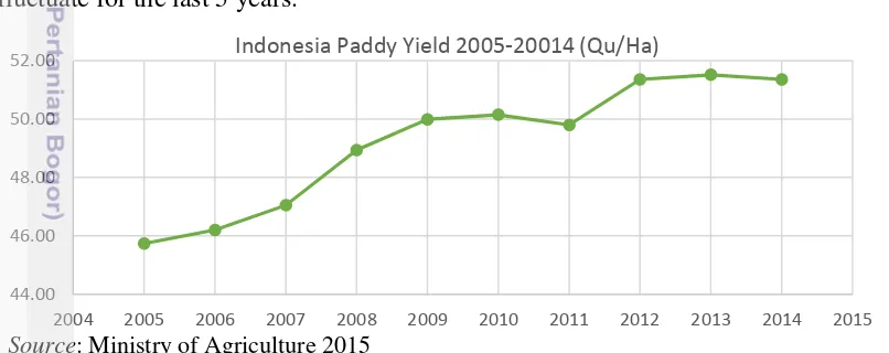
9 Indonesian paddy yield 2005 – 2014 (Qu/Ha) 23
10 Impulse Response Function result; response of paddy production
towards shock on temperature changes 28
11 Impulse Response Function result; response of rice price towards
shock on temperature changes 29
12 Impulse Response Function result: respones of rice price volatility
towards shock on temperature changes 29
13 FEVD (Variance Decomposition Approach) result of domestic rice
price variable 30
14 FEVD (Variance Decomposition Approach) result of Indonesian rice
price volatility variable 31
LIST OF APPENDICES
1 Stationarity test for ARCH-GARCH model 37
2 Correlogram test for Indonesian rice price variable 37 3 Best ARIMA model for Indonesian rice price variable 38
4 ARCH test for Indonesian rice price variable 38
5 Best ARCH-GARCH model 39
6 Stationarity test for VAR/VECM variables 39
7 VAR stability testing 42
8 Optimum Lag testing 43
9 Cointegration test result 43
10 VECM driving factors of Indonesian rice price 44
11 FEVD result 48
1
Source : FAO 2014
Figure 1 Development of World Food Price Index
1
INTRODUCTION
Background
In recent years, there has been food security issue growing along with the emergence problems called 3F-crisis (food, fuel, and financial crisis) as the spillover effects of 2008 global crisis. This phenomenon resulted in food prices surge at the consumer level around the world. Figure 1 shows the rise in world food price index and largely dominated by the rising prices of cereals. Based on World Bank Trade Sector Development report(World Bank 2011) from the sub-indices of international food prices, the price of grain increased dramatically (in the last 30 years) starting on the late 2007 and reach its peak at the early period of 2008 crisis.
One of grain commodities affected by price fluctuations due to 2008 global crisis is rice. Unlike corn and wheat, rice is not used to produce biofuels. Nevertheless, the rise in grains price to another one has led to rapid increase in the price of rice over the past decades (World Bank 2011). In terms of supply, production of paddy (rice) in the world ranks third of all cereal after maize and wheat (FAO 2014). Most of the rice granary of the world comes from Asian countries with Indonesia in the third position after China and India. Following graph show the rice (paddy) main producing countries in 2012.
Source: FAO 2014
Figure 2 Main producing countries of rice (paddy) 2012
-2
The fact was all of these main producer countries also had large consumption of rice as its staple food. As a result, only a small fraction of the world's rice production is traded between countries (5-6% of total world production) because each country must meet their domestic needs. Indonesia's own position is the world's largest rice importer as 14% of the rice traded in the world (Indonesian Ministry of Trade 2012). Indonesia’s per capita rice consumption recorded still quite high, reaching averagely 6.18 kg a week or 139.15 kg/capita/year (BPS 2014). This value is much higher than the ideal consumption by the developed countries standards as 80-90 kg/capita/year.
Meanwhile, climate change and weather variability are the two climate anomaly phenomenon which is now a strategic issue and a serious concern because it is believed to have had a big impact to life in various sectors. This statement can be proved by the facts that there has been an increase number of floods and periods of drought, devastating cyclones, water, soil and land resources that are continuing to decline in several parts of the World on the last decades (IRRI 2006). The IPCC 4th Assessment Report (IPCC 2007) states that Southeast Asia is expected to be seriously affected by the adverse impacts of climate change. It is projected that by 2100 the annual mean temperature in Indonesia, the Philippines, Thailand and Viet Nam are going to rise by 4.8 °C, with the global mean sea level will increase by 70 cm during the same period (ADB 2009). Since most of its economy relies on agriculture and natural resources as primary income, climate change has been and will continue to be a critical factor affecting productivity in the region mentioned before.
Indonesia itself is predicted to experience temperature increases of approximately 0.8°C by 2030, while the rainfall patterns are predicted to change, with the rainy season ending earlier and the length of the rainy season becoming shorter (FPRI 2011). Some empirical studies has been done to analyze this phenomenon. Climate change affects all economic sectors, but the agricultural sector is generally the hardest hit in terms of the number of poor affected (Oktaviani 2011). There has been changes in precipitation and cycles of droughts and floods triggered by the Australasia monsoon and by the El Niño Southern Oscillation (ENSO) for the past three decades in Indonesia (Naylor R. L. 2007; Boer 2010). Thus, this has led to agricultural production damage, causing negative consequences for rural incomes, food prices, and food security in Indonesia. In Indonesia case, rice is one of the most important staple foods for more than half of the world’s population (IRRI 2006) and influences the livelihoods and economies of billions people in Asia. A recent study by the International Food Policy Research Institute (IFPRI), titled ‘Climate change: Impact on agriculture and costs of adaptation’, highlighted some of the anticipated costs of climate change, which one of them is the increase prices in 2050 by 90% for wheat, 12% for rice and 35% for maize on top of already higher prices.
Problem Identification
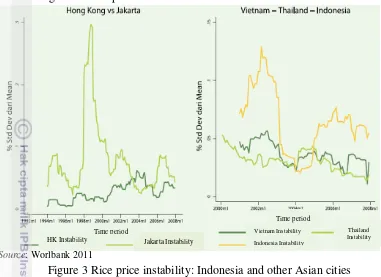
3 shows the instability of the local rice price in Indonesia compare to other Asian cities after 2008 global food spike.
Source: Worlbank 2011
Figure 3 Rice price instability: Indonesia and other Asian cities
Based on the Figure 3, we can see the instability of Indonesia’s price of rice reached the highest level compare to other major rice producer’s countries (Thailand and Viet Nam). In time of 2008 crisis too, the level of Jakarta rice price instability reach the highest spike compared with Hongkong as the non-major rice producing country.
The rice instability both in terms of price, stock, and production will gradually affect social and economic instability, also political security in each country. Since the biggest food consumption of Indonesian people is rice, then it became main concern if the price becames fluctuated, especially after the last food price spike. Therefore the first question that should be answered in this thesis will be “How was the volatility of domestic rice-price in Indonesia after 2007-2008 crisis?”
Despite the large literature has examined local food prices in developing countries, there is limited systematic evidence on the relationship between domestic weather disturbances and local food prices, especially in Indonesia. Although the effects of climate change already became such a reality in Indonesia, however to date there has few studies that have assessed the impacts of current and forecast future climate change on the agricultural economic variables. Therefore, the next question would be “What are the main drivers of fluctuating local rice price in Indonesia?” and “How far this climate change variables (especially temperature changes) affect Indonesia local rice price and its paddy production?”
Objectives
The primary objective of this research is to calculate the fluctuation (the volatility) of Indonesian rice price, then to investigate what are the main drivers that causing the fluctuation of local rice price in Indonesia; and the last one is to
HK Instability Jakarta Instability Time period
Indonesia Instability
Thailand Instability Vietnam Instability
4
investigate the consequences of climate change variables (especially temperature changes) towards Indonesian paddy production, local rice price, and its fluctuation (volatility).
Significance
This thesis makes a contribution to the existing empirical literature by combining the two lines of empirical research in an emerging area of green economics using relatively new time series methodologies that overcome some of the methodological concerns of other studies (e.g estimating price volatility using ARCH-GARCH, testing for cointegration test to find out the relationship between the agriculture economics variables). Finally, the empirical results of this single country study may be helpful in guiding policy makers in devising long term sustainable agricultural economics policy in Indonesia.
Research Coverage
This research was conducted in the national scope. The object in this study covers only single food commodities, rice. The data type used is a monthly time series data from January 2007 until December 2014.
The price of rice used in this study is medium retail price of rice which sold in major traditional markets in Indonesia, not the producer price or the Government purchasing price (HPP). This study did not distinguish the price of rice according to the quality and type, but rather use the number of rice commodities being produced data (i.e: paddy-production variable, the Government's rice reserve variable) and any other appropriate data.
International trade variable used here is the world rice price. While the trade policy such as export and import tariffs are not used as explanatory variables in this research modelling because the data is not available in the monthly period. The Indonesian macroeconomic indicators used in this research are the inflation, household consumption, exchange rate, and the interest rate. Also, due to the limited availability of monthly data, the climate change indicators used in this study was the change in temperature which using ENSO 3.4 temperature variable.
2
LITERATURE REVIEW
Food Price Volatility
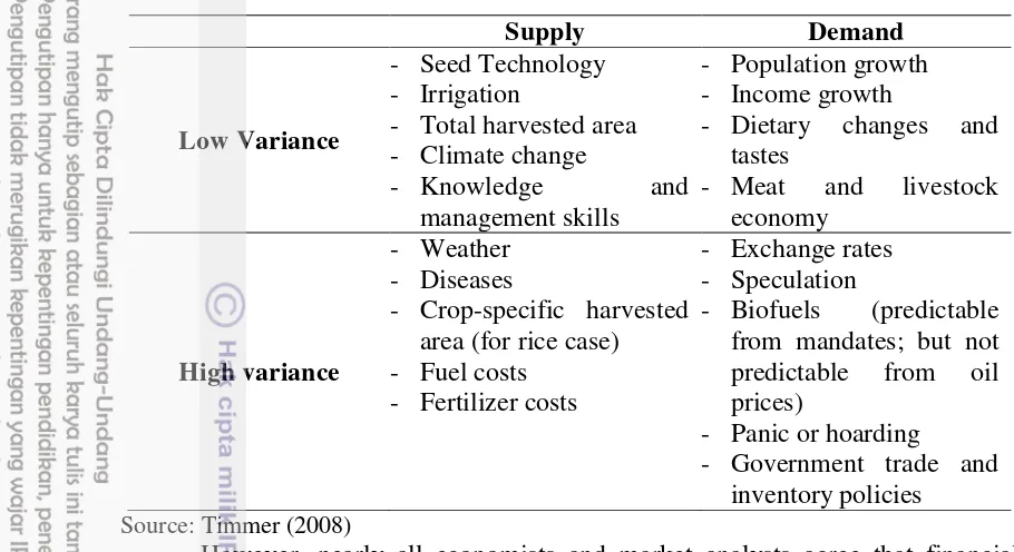
5 a commodities as agricultural commodities. Food price volatility that happening in the foods market does not happen by itself, they surely get influenced by any other factors. It is useful to think about the factors causing high and volatile food prices in terms of cumulative layers of causation (Timmer 2008). Following are the four basic drivers that seem to be stimulating rapid growth in demand for world food commodities:
1. Rising living standards in China, India, and other rapidly growing developing countries lead to increased demand for improved diets, especially greater consumption of vegetable oils and livestock products (and the feedstuffs to produce them). China is a major importer of soybeans for both meal and oil and India is a significant importer of vegetable oils. However, wheat and rice consumption in the China and India are not rising significantly and both countries are largely self-sufficient in both commodities.
2. The rapid depreciation of the dollar against the euro and some other important currencies drives up the price of commodities quoted in dollars for both supply and demand reasons. The depreciation of the dollar also causes investors “long” in dollars (i.e., most US-based investors, but holders of dollars globally as well) to seek hedges against this loss of value, with commodities being one attractive option.
3. Mandates for corn-based ethanol in the US (and biodiesel fuels from vegetable oils in Europe) cause ripple effects beyond the corn economy, which are stimulated by inter-commodity linkages (Naylor 2007; Timmer, Falcon, and Pearson 1983). There is active debate about whether legislative mandates or high oil prices are driving investments in biofuel capacity (Abbot, Hurt, and Tyner 2008), but no doubt about the increasing quantities of corn and vegetable oil being used as biofuel feedstocks (Elliott 2008). 4. Massive speculation from new financial players searching for better returns
than in stocks or real estate has flooded into commodity markets. The economics and finance communities are unable to say with any confidence what the price impact of this speculation has been, but virtually all of it has been a bet on higher prices.
6
Table 1 Supply and demand drivers of fluctuating food price
Supply Demand
However, nearly all economists and market analysts agree that financial speculation cannot drive up prices in the long run—over a decade or longer. Only the fundamentals of supply and demand can do that (Timmer 2008)
Food Price Stabilization
World food price volatility is inevitable things since more than three decades it has never happened. The food crisis of 2007/2008 and 2010/2011 is the culmination of the rise in food prices. Price volatility also can not be avoided in agricultural commodities markets. Price volatility cannot be removed, but can be minimised its impact through a variety of policies both local and international. According to Timmer (2011), there is some policy to cope with the volatility of food prices. Price stabilization policy can be one of the alternatives to reduce volatility, but in the implementation is often fail. The price stabilization were failed because it could not be completed efficiently and effectively. Stabilization policy price policy type is the most widely chosen by countries affected by price shocks. According to the World Bank (2010) from 56 countries surveyed, 23 countries choose to implement a policy of stabilization the price for tackling the problem of price uncertainty. These policies are not efficient. Mongolia and Zimbabwe is an example of two countries that implement a stabilization of prices but losses against the manufacturer because the manufacturer sells its products below market price.
7 Policies to cope with price volatility can also be done by separating the roles of Government and the private sector. The Government role is to enforce the law and institutions so that the private companies can reduce risk price uncertainty. Other important policies to reduce volatility are the information disclosure and market agricultural development policy give priority to the improvement of income especially in rural (Tangermann 2011).
The availability of food reserves for domestic needs is another way to cope with price volatility (Timmer 2011; Tangermann 2011). Each state either the exporter or the importer should have a backup food, so as to prevent prices rising sharply. The world food stock should be realized simultaneously and is part of international cooperation (Timmer 2011). There are three types of good food reserves domestic and international, namely (1) the national food reserve that is useful for importing countries when food prices are very high and not allows for the purchase of food, (2) international food reserves managed by international organizations and in some locations aims to provide a food reserve for the developing countries not prepared to face extreme food crisis, and (3) international institutions like the International Grain Clearing Arrangements (IGCA) should be able to be proponents of food reserves for countries exporters in countries failed exports.
Climate Change, Climate Variability, and ENSO
Climate is "average" weather condition for a given place or a region. It defines typical weather conditions for a given area based on long-term averages. Compare to weather, climate contains statistical information, a synthesis of weather variation focusing on a specific area for a specified interval. Climate is usually based on the weather in one locality averaged for at least 30 years. Climate change is a phenomenon where there is changes in atmosphere composition that will enlarge the observed climate variability during such long periods (Trenberth 1996).
Climate variability is the fluctuation of climate elements that occur in a certain span of time as seasonal or annual variation (i.e: rainy season and the dry season shifting, changes of timing, or its duration) as well as extreme climate events. Climate variability describes short-term changes in climate that take place over months, seasons and years. This variability is the result of natural, large-scale features of the climate that we looked at earlier.
8
Source : NOAA, http://www.pmel.noaa.gov/tao/elnino/nino-home.html
Figure 4 Three-dimensional depiction of three important phases of the El Niño-Southern Oscillation (ENSO): Normal (left), La Niña (centre) and El Niño (right)
Normal condition, or the neutral phase of ENSO, is shown on the left in Figure 4. The trade winds (white arrows) blow to the west and cause a build up of warm surface water (orange-red areas) and higher sea level in the West Pacific. The warm water heats the air above it, making the moist air rise and forming clouds (this is called convection). This warmer air then moves east to where the air is cooler, the cooler air sinks towards the surface and moves west, creating a convective circulation.
Indonesia climate variability is very closely related to the El Niño Southern Oscillation (ENSO) in the Pacific Ocean (Naylor 2002) and the Indian Ocean Dipole (IOD) in the Indian Ocean (Ashok 2001; Mulyana 2001). Influence of ENSO in Indonesia is not the same on each area. However, the influence of ENSO is very great on any area that has a monsoon rains patterns, small influence on the area rain with equatorial pattern and not clear on local rainfall patterns (Boer 2002).
When El Nino condition happens, the temperature of the sea level in Indonesia and around is cooling down. As a result, the air mass flowhot bottom moves from Indonesia headed towards the East. As the area of subsidence, then the rainfall in Indonesia is relatively below normal. The condition became vice-versa when La Nina happens, where the flow of hot air masses moving down from the tropical Pacific to Indonesia. As the result, there is strong convective rainfall that relatively above normal in Indonesia. As an indicator for monitoring the events, the commonly used data measurement of Indonesia’s SLP is the NINO 3.4 (170°WL-120°WL, 5°SL-5°NL), in which the positive anomalies indicate the occurrence of El Nino, whereas the negatives anomalies characterized the La-Nina Phenomenon.
9 Theoretical Framework
Price Formation Model
Understanding the cause of price fluctuation (or volatility) implies an empirically refutable model of mechanisms of action. As for food prices, this means an analytical model based on supply and demand mechanisms with equilibrium prices derived from basic competitive forces. This should be explained in order to understanding the contribution a wide range of basic causes of fluctuating prices by important food commodities—rice, wheat, corn, and palm oil. Some of these causes may be exogenous, (e.g., weather shocks or legislated mandates for biofuel usage). But many will be endogenous, (e.g., responses of producers and consumers to prices themselves, perhaps even policy responses of governments to prices).
The model of price formation developed here attempts to incorporate all of these factors in a rigorous enough way to bring data to bear on answering the key question in this research. Consider the most basic model of commodity price formation that is capable of illuminating our problem.
= � , , �− , = � � �−� (1)
= � , , �− , = � �− (2)
where Dt = demand for the commodity during time t; St = supply of the commodity during time t; f and g = functional forms for demand and supply functions, respectively; = time-dependent shifters of the demand curve; = time-dependent shifters of the supply curve; � = equilibrium market price during time t; �− = market price during some previous time period t-n; and, , , and = indicators that demand and supply responses will vary depending on whether they are in the short run (sr) or long run (lr). In the specification below, these will be short-run and long-short-run supply and demand elasticities.
Meanwhile, in short run equilibrium, = . Then, assume the demand and supply functions are Cobb-Douglas (in order to simplify the supply and demand elasticities).
log + log � + log�− = log + log � + log�− (3)
Then, solving for the equilibrium price P:
log � =[log − log ][
�− ] + log�− [ − ]/ [ − ] (4)
The next step is taking its first differences to see the factors that explain a change in price from − to time period which reveals such a complicated result:
log � ={[log − log −1]−[log − log −1]}
[ �− ] + [log�− − log�− + ] [ − ] [ − ]⁄ (5)
10
This is what we are trying to explain. What “causes” changes in log �? Why are the food prices high? Answering these questions, we have to simplify the equation. Let SR = the net short-run supply and demand respons − , which is always negative because <0 and < . Let LR = the net long-run supply and demand response − , which is always positive, for similar reasons (note that the demand coefficient is subtracted from the supply coefficient in this case, the opposite from the short-run coefficients above). Let log = log − log − , which for small changes is the percentage change in the supply shifters. Let
log = log − log − , which for small changes is the percentage change in the
demand shifters. Finally, let log�− = log�− − log�− + , which for small changes is the percentage change in the commodity price for some specified number of time periods in the past, for example, 5 or 10 years (after which the long-run producer and consumer responses to price have been realized).Combining all of these new definitions, we have a simpler equation explaining percentage changes in commodity prices:
% ℎ � � =[% ℎ � −% ℎ � ]+ [% ℎ � �− ]� / (6) The results show how simple the answer appears to be. There are four key drivers:
1. The relative size of changes in to , i.e., factors shifting the demand curve relative to factors shifting the supply curve;
2. The relative size of short-run supply and demand elasticities ( and ); 3. The relative size of long-run supply and demand elasticities ( and ; and 4. How large the price change was in earlier time periods
Over long periods of time, the first driver is clearly most important—how fast is the demand curve shifting relative to the supply curve? At the level of generality specified in this model, the actual underlying causes of these shifts do not matter. All that matters is the net result. The “simple” fact is that commodity price changes are driven by the net of aggregate supply and demand trends, not their composition.
It is important to realize that the analytical model of price formation makes a sharp distinction between factors that shift the demand and supply curves (the in and coefficients), and the responsiveness of farmers and consumers to changes in the market price (the and coefficients), which show up as movements along the supply and demand curve. Analytically, the distinction is very clear, but empirically it is often hard to tell the difference. If farmers use more fertilizer in response to higher grain prices, should this count as part of the supply response or as a supply shifter? If governments and donor agencies restrict their funding of agricultural research because of low grain prices, is the resulting lower productivity potential a smaller supply shifter a decade later or a long-run response to prices? Whatever the labels, it is important to understand the causes.
Therefore, below are the lists of possible factors that causing high food prices fluctuation (Timmer 2008). For demand, it includes (based on its predictability): 1. Population (driven by demographic transition, fertility, mortality, famine) 2. Income growth (driven by economic policy, trade, technology, governance)
a. Direct consumption
11 3. Income distribution (driven by globalization, food prices, agricultural growth,
structural transformation)
4. Biofuel demands (driven by political mandates and the price of petroleum) a. Direct demand for maize and vegetable oils
b. Ripple effects on other commodities
5. US dollar depreciation (most commodities on world markets are priced in dollars)
6. Food prices (endogenous, driven by supply/demand balance and technical change; impact felt through the demand elasticities)
7. Private stockholding
a. Commercial (driven by price expectations and supply of storage) b. Household (driven by price panics and hoarding)
8. Public stockholding (driven by buffer stock policy) a. Trade policy
b. Procurement policy 9. Financial speculation
a. Futures/options markets and “sophisticated” speculators b. Role of commodity index funds available to general investors
Meanwhile for supply, the list is not so long, but the factors may be even more difficult to understand and quantify:
1. Area expansion
a. Irrigation and cost of water
b. Deforestation and environmental costs
c. “Benign” area expansion in Africa and Latin America? 2. Yield growth
a. Availability and costs of inputs (i.e: Fertilizer costs, Energy costs, and Sustainability issues)
b. Seed technology and the Genetic Modified Organism (GMO) debate c. Management improvements/farmer knowledge
3. Variability a. Weather
b. Climate change
Empiricial Review
12
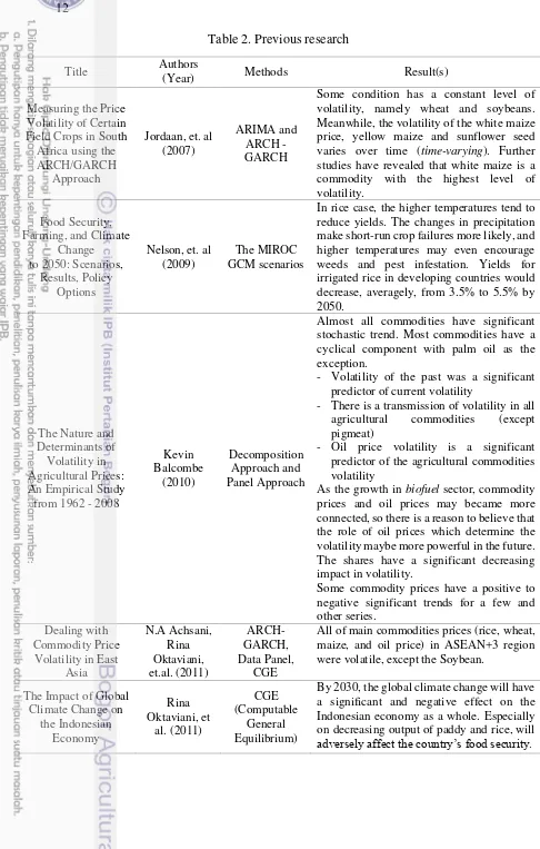
Table 2. Previous research
Title Authors (Year) Methods Result(s)
Measuring the Price volatility, namely wheat and soybeans. Meanwhile, the volatility of the white maize price, yellow maize and sunflower seed
In rice case, the higher temperatures tend to reduce yields. The changes in precipitation make short-run crop failures more likely, and higher temperatures may even encourage weeds and pest infestation. Yields for irrigated rice in developing countries would decrease, averagely, from 3.5% to 5.5% by
Almost all commodities have significant stochastic trend. Most commodities have a cyclical component with palm oil as the exception.
- Volatility of the past was a significant predictor of current volatility
- There is a transmission of volatility in all agricultural commodities (except pigmeat)
- Oil price volatility is a significant predictor of the agricultural commodities volatility
As the growth in biofuel sector, commodity prices and oil prices may became more connected, so there is a reason to believe that the role of oil prices which determine the volatility maybe more powerful in the future. The shares have a significant decreasing
All of main commodities prices (rice, wheat, maize, and oil price) in ASEAN+3 region
13
Despite the large literature that has examined local food prices in developing countries mentioned in the previous studies on the Table 2, however there is limited systematic evidence on the relationship between domestic weather disturbances and local food prices fluctuation especially the staple food prices. In Indonesia, rice as one of the staple food plays important role to the economic stability. Therefore, this research focusing on measuring the rice price fluctuation and its relationship between the temperature change and other driving factors behind its fluctuation.
Logical Framework
The issue of food security as the spillover effects of the global crisis of 2007-2008 resulted food price spikes at the consumer level around the world. Rising food prices have become a burden for the poors in developing countries who spend on average half of their household income on food, especially on cereal commodities. Meanwhile, in the last decades, there have been an increase number of floods and periods of drought, devastating cyclones, water, soil and land resources that are continuing to decline in several parts of the world. Southeast Asia is expected to be seriously affected by the adverse impacts of climate change. There have been changes in precipitation and cycles of droughts and floods triggered by the Australasia monsoon and by the El Niño Southern Oscillation (ENSO) for the past three decades in Indonesia. This has led to agricultural production damage, and probably would causing negative consequences for rural incomes, food prices, and food security in Indonesia. Since most of Indonesia economy relies on agriculture and natural resources as primary income, climate change has been and will always continue to be a critical factor affecting productivity in the region. In Indonesia, rice act as one of the staple food products that has strategic role in strengthening food security, economic security and the political stability of this country. Indonesia's own position is the world's largest rice importer (14% of the rice traded in the world). Rice market The Challenges of
Romanian domestic sugar market is volatile, as well as World Sugar market. Romania’s current volatility context is a mixture between imported volatility, internal instability and lack of maturity of its market structures.
The global rice trade activity is low and tend to self-perpetuate thus they does not cause
14
itself in world trade is a “thin” commodity (slightly traded). This causes the price in world rice market and other rice producer countries might be volatile. Therefore the first aim of this research is to calculate the fluctuation of Indonesian rice price (the volatility) especially after the 2007-2008 crisis up until the newest periods and its drivers factors behinds it. Despite the large literature that has examined local food prices in developing countries, there is limited systematic evidence on the relationship between domestic weather disturbances and local food prices. Thus the next aims of this study it to analye does climate change became as one of the driving factor behind the rice-price fluctuation, and how much this temperature changes affect Indonesia paddy production. Following the logical framework of this study.
= Scope of study
Is the Indonesian rice price volatile during these period?
(Analyse using ARCH-GARCH)
RICE
Specifically, how far climate change variable (especially temperature changes) affect Indonesian rice-price volatility?
Also, how much this temperature changes affect Indonesia paddy production and local rice price?
(Analyse using IRF and FEVD)
If Yes, What are the driving factors affecting the Indonesian Rice Price Volatility? (Analyse using VAR/VECM)
1. Domestic (local) rice price
7. Climate change variable (Temperature changes) 8. Interest rate
9. Consumer Price Index (CPI)
3F Crisis (Food, Fuel, Financial)
after 2007-2008 global crisis Trigger Food Security Issue proved by the food price spikes, especially on cereal commodities
Policy Implication in Indonesia Bio-fuel issue and Climate
Change phenomenon
15
3
RESEARCH METHODOLOGY
Data and Sources
This study is based on monthly time series data covering the time period from January 2007 to December 2014. This particular period was chosen because of the existence of 2007-2008 global price spikes over agricultural products (domestically and internationally). The main variable used here is the local rice price (nominal price) Indonesian which published monthly as consumer retail price whose taken from main traditional markets all over the provinces in Indonesia. Its unit value is in Rupiah/Kg. Based on previous research, following are factors that might affect the fluctuation in Indonesia local rice prices including:
a. Paddy Production
Rising and fluctuating the prices of rice caused by the production of paddy and consumption of rice that varies. The presence of paddy production and rice consumption shocks are caused by the elasticity of supply and demand could lead to price volatility (Gilbert and Morgan 2010; HLPE 2011; Braun and Tadesse 2012). Since the rice still became main staple food in Indonesia, thus its demand elatisticity does not play a significant matter in rice price formation. Now it really depends on the supply side which is the paddy production itself.
b. Domestic Stock
Other factors that cause volatility of food prices is domestic stock (Gilbert and Morgan 2010; Tothova 2011; FAO 2011). Stock food the world has been experiencing a decline since ten years ago, but the stock of material staple food of the world relative to the use of the lowest decline in 2006 and 2008. World food stock decline caused by several factors such as growth, the decline in agricultural commodities due to productivity and low prices, besides policy changes in stock the farm established by the EU and China also affects world food stockpiles low (Tangermann 2011).
c. World Food Prices (in this case World Rice Price)
World food prices is one of the factors that affect domestic food prices as it has been discussed in many studies (ADB 2009). This shows the linkages between the domestic market and international market. Although domestic does not do the food commodities for import, then the world food prices has increased, then the world food price increases would be able to affect domestic food prices. With the law of one price, known as Purchasing Power Parity (PPP), for which this law states that the same goods will be sold at the same price at the same time with different places (Krugman 2009). The law assumes that there are no obstacles in the trade that caused the domestic price and the world price being different. From the explanation above, it can be concluded that there is a positive relationship between world food prices with domestic food prices.
d. Household Consumption
16
However, if the supply of food commodities has not changed, then with an increase in demand for food, will lead to increased food prices and allow the occurrence of fluctuations in food prices. It can be concluded that the per capita income has a positive relationship with changes in food prices.
e. Exchange Rate
Domestic food availability may not only come from domestic production, but also come from abroad. When the exchange rate of Indonesia get appreciated, then the world's food prices are relatively cheaper when compared with its domestic price (Balcombe 2010), so that would cause a wave of imports that will lead to increased availability of domestic food. When excess domestic availability, then domestic food prices will also decline.
f. Climate Variable
In some of previous research that has been done before, the climate change phenomenon such as El Nino and La Nina has a significant impact towards commodity prices (Brunner 2000). In this research, climate factor that will be used is an index that measures the occurrence of El Nino phenomenon, a phenomenon of which increasing surface temperature in the Pacific Ocean. During this El Nino phenomenon, the beginning of the rainy season is going to be slower and the drought that is capable of lowering the production of food commodities that hung from a very good system of irrigation. This will affect the domestic supply of the main food commodities Indonesia and able to affect change in price.
g. Interest Rate
The interest rate is one of the factors of macroeconomic variables that have a direct impact on the price of commodities, where the interest rate is a measure that is capable of describing the return from stocks. In addition, the interest rate is also an important indicator that describes the State of the economy. Interest rate fluctuation that occurred indicating the uncertainty of economic conditions and its ability to affect commodity prices, including food commodities (Balcombe 2009; Roache 2010). h. Consumer Price Index (CPI)
The CPI is meant to indicate average fluctuations in prices of commodities (goods and services) purchased by households nationwide. In other words, using the consumption by households at a given time as the reference period, the index shows changes in the total amount of expenditure required to purchase the equivalent goods and services purchased by households in the reference period, setting the consumption structure. Thus, the CPI is intended to measure changes in prices themselves. So, the changes in CPI may lead to the changes in food prices and in this case the rice price itself.
17 Table 3 List of variables
Variable names Unit Symbol Source
Indonesia rice price
Domestic Stock of Rice Ton LnDomStock Indonesia Public Stockholding (BULOG)
Household Consumption Bill. Rp Ln_HHCONS Bank Indonesia World Rice Price $/mt Ln_WorldPrice Pink Sheet World Bank
Temperature (ENSO 3.4) ° C TEMP Climate Prediction Center (CPC) Exchange Rate USD/Rp LN_ER Bank Indonesia
Interest Rate % BIRate Bank Indonesia
Consumer Price Index - CPI Indonesia
Central Statistical Bureau (BPS)
Methodological Frameworks
ARCH-GARCH Model
The need for accurately assessing price volatility appears especially from the high level of risk and uncertainty that creates for producers, consumers and policymaker’s worldwide (Popa et.al 2013). The modeling of volatility in time series has been revolutionized by the introduction of the Autoregressive Conditional Heteroskedasticity (ARCH) models by (Engle 1987) and their generalized form (GARCH) by (Bollerslev 1986). Numerous authors, as for example (Jordaan 2007), Pop and Ban (2011), argue in favor of GARCH models on the grounds that they have the merit of accounting for both the predictable and unpredictable components in the price process, being also capable of capturing various dynamic structures of conditional variance.
The volatility (fluctuation) is reflected in the residual variance that does not meet the homoscedasticity assumptions (Firdaus 2011.) Volatility based models ARCH (m) assumes that the data variance fluctuations are influenced by a number of “m” data fluctuations before. GARCH (r, m) assumes that the data variance fluctuations influenced by a number of previous m data fluctuation and volatility of the previous amount of data r. The following is the general form GARCH (r, m) in this study:
ℎ =K+ ℎ− + ℎ− + ⋯ + ℎ − + − + − + ⋯ + − (7)
In its general form above, a GARCH (r, m) model includes two equations, one for conditional mean and one for conditional variance. The coefficients of ARCH-terms − reveal the volatility of previous periods of time, measured with the aid of squared residuals from the equation of mean, and the coefficients of GARCH-terms
18
are being estimated; , … , is coefficient of orde r that are being estimated. Having obtained the best model of ARCH-GARCH, then the following model is used to estimate the value of future volatility (ζt− ) from an economic variable, where t = √ℎ . Forecasting variety of ARCH (m) for the upcoming period is formulated as follows:
ℎ = + − + − + ⋯ + − (8)
VAR/VECM Model
VAR modeling is a form of modeling used for multivariate time series in which exogenous and endogenous variables became indistinguishable because in this modelling all the variables became endogenous (variables whose value is determined in the model). In accordance with Sims (1972), the variables used in the VAR equation selected based on relevant economic theory and only endogenous variables included in the analysis. This economics model was chosen because it meets four important things to be obtained from the establishment of economic modelling, namely: data description, forecasting, structural inference, and policy analysis. The VAR model can be written in the following mathematical form:
= + ∑= − + � (9)
where:
= Vector of dependent variable (n x 1)
= Vector of exogen variables including Constanta (intersep) and trend (n x1) = Number of lag, or ordo for the VAR model
� = Vector of Error term (n x 1)
= Matrix of parameter, size n x n for each i = 1, 2 …
VAR / VECM model that created by Sims (1972) basically provides a tool for the 4 kind of quantitative analysis: a) Forecasting; b) Granger Causality Test; c) Impulse Response Function (IRF); d) Forecast Error Decomposition of Variance (FEDV). According previous research (Akhmat, 2014), the following sequential procedures are adopted as part of this methodology.
In order to confirm the degree; we execute unit-root stationarity tests. The Augmented Dickey–Fuller (ADF) is suitable testing procedure that is based on the null hypothesis that a unit root exists in the autoregressive representation of the time series. This because the time series data is often plagued with non-stationarity in levels, hence, the estimation based on such series usually provide spurious results (Azhar 2014). Dickey and Fuller (1979) devised a procedure to formally test for non-stationarity which does not take into account high order auto correlation and hence limits the power of the test. The Augmented Dickey–Fuller (ADF) test have a null hypothesis of non-stationarity against an alternative of stationarity. The next step is choosing the optimal lag length for all the variables in non-differenced data. This VAR model should be estimated for a large number of lags, then reducing down by re-estimating the model for one lag less until we reach zero lags. In each of these models, we inspect the values of Akike Information Criteria (AIC) and the Schwarz Information Criteria (SIC) criteria.
19 integrated and are of the same order, it implies co-integration (Pesaran 2001). In the second step, Johansen' cointegration tests are applied on the series of same order of integration i.e. I(1) series which determine the long run relationship between the variables. When the series that are co- integrated are of order 1, a trace test (Johansen's approach) indicates a unique cointegrating vector of order 1 and hence indicates the long run relationship. In the multivariate case, if the I (1) variables are linked by more than one co-integrating vector, the Granger causality (Engle 1987) procedure is not applicable. The Johansen and Juselius method has been developed in part by the literature available in the field and reduced rank regression. Johansen and Juselius (Johansen 1990) propose that the multivariate co-integration methodology can be defined in the following general VAR model form:
Volatt= (LnDomRicet,LnProductiont,LnDomStockt,LnHHConst,LnWorldRicet,
Tempt,LnERt BIRatetCPIt) (10)
While the matrix form for the general VAR model in this research is following:
[ as the lag coefficient of j-variables for the-i equation.
This study investigates the factors that affects the fluctuating rice price then investigate the influence of climate change variables on rice price and its volatility from two perspective. One is to conduct the Johansen cointegra-tion tests to explore the influencing directions between these factors that affects the rice price fluctuation mentioned in the general VAR model above respectively. The other is to compare the influencing magnitude of climate change variable on rice price, paddy production, and its volatility based on the Vector Error Correction Model (VECM), Impulse Response Function (IRF) and variance decomposition approach (FEVD). VECM itself is a form of VAR that being restricted (restricted VAR). This additional restriction should be granted because of the existence of not stationary data but co-integrated. If the data is not stationary in levels but being stationary at its difference, then it must be examined whether the data used in the model has a long-term relationship or not. The existence or absence of a long-term relationship between the variables in the VAR system can be determined by performing cointegration test. If there is cointegration, the model used would be Vector Error Correction Model (VECM). VECM specification restricted the long-term relationship endogenous variables that converge into its cointegration relationship, but still allow the existence of short-term dynamics. Hereby the general mathematical form of VECM:
20
Following is the VECM model used in this study (matrix form):
[ lag coefficient of j-variables for the-i equation. Following are the explanation of each variables used in this model:
Volat = Indonesian rice price volatility which estimated by ARCH- GARCH
LnDomRice = Indonesian monthly domestic rice price (consumer retail price), its unit value is in Rupiah/Kg and nominal price
LnProduction = Indonesian monthly paddy production (national), gotten from Indonesia Central Statistic Bureau. Its unit value is in Quintal. LnWorldRice = World monthly rice price (f.o.b price) published by The Commodity Pink Sheet World Bank. Its unit value is in metric ton (MT)
LnHhCons = Household Consumption, monthly basis, with its unit value in billion Rupiah. Source from Indonesia Central Bank (BI) LnDomstock = National public stock of rice, organized and published of
BULOG (Indonesia’s Public Stockholding) on monthly basis. Its unit value is in Ton
CPI = Consumer Price Index, monthly index published by Indonesia Central Statistic Bureau
LnER = The Rupiah to US dollars exchange rate whose value taken at the end of each period (monthly). Source from Indonesia Central Bank (BI)
Temp = Monthly El Niño Southern Oscillation (ENSO) Index NINO In this reseach, we use it as temperature proxy, gotten from US Climate Prediction Center (CPC)
21
4
RESULT AND DISCUSSION
World and Indonesia Rice Market Overview
As an overview of Indonesia rice markets, following Figure 6 is the Indonesia rice price evolution from the early 2007 to the last period of May 2015.
It can be seen the prices continue to move up slowly starting at the end of 2009 and keeps fluctuating with the increasing trends. This is something different from the international rice price condition as it reported by the World Bank (2011) that there was high spike in world rice prices on April and May 2008 which the world rice price reach even three times higher than the normal price (became 900 US $/ MT). While in mid-2009 and thereafter, the world price relatively became stable with a new price equilibrium (as compared to 2007 and earlier), in the range of US $ 500-600/MT/month (Figure 7).
Source: Indonesia Central Statistic Bureau 2015
Figure 6 Indonesian consumer retail price of rice January 2007 – May 2015 0
Indonesia Consumer Retail Price of Rice (Rp/Kg)
0
International Prices of Rice, Thailand (Bangkok) (5% broken) (USD/tonne)
Source: The World Bank 2015
22
ARCH-GARCH Model Specifications
In the specification of ARCH-GARCH models to measure rice price volatility, there are 2 main stages: 1) Identification and model determination (mean equation); 2) Identification and determination of ARCH-GARCH models. Stage (1) includes testing data stationery, determining a tentative ARIMA models to estimate the parameters and selection of best model. The following table shows the results:
Table 4 ARCH-GARCH model specification result
*) Level of significance 5%
Based on the Table 4, Indonesian rice prices has the ARCH effect. This is shown in prob.F value which greater than the critical value 0.05. This means the applications of ARCH-GARCH models can be done for measuring Indonesia rice price volatility. This measure of volatility is then shown by the conditional standard deviation which is root of variance of the ARCH-GARCH best selected models which had estimated.
The Volatility of Indonesia Domestic Rice Price
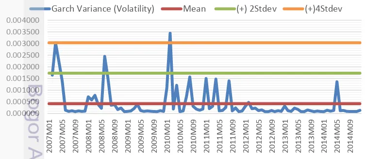
Based on author’s estimation result using Eviews 8, Indonesian rice price volatility values over time shows the variation (time varying) from 2007 to 2014, as we can see in Figure 8.
Garch Variance (Volatility) Mean (+) 2Stdev (+)4Stdev
23
44.00 46.00 48.00 50.00 52.00
2004 2005 2006 2007 2008 2009 2010 2011 2012 2013 2014 2015
Indonesia Paddy Yield 2005-20014 (Qu/Ha)
Source: Ministry of Agriculture 2015
Figure 9 Indonesian paddy yield 2005 – 2014 (Qu/Ha)
Based on Figure 8, the Indonesia rice price volatility moving along above its mean on some periods, such as: on the early 2007; the first quarter of 2008; early 2010 until the end of 2011; and the last March 2014. The Indonesian rice price volatility reach its peak on the early 2010 and continue to fluctuate until last quarter of 2011. The first peak (January 2010), reach up until more than 4 times its standard deviation. Then between the periods of March 2010 until September 2011, it slowly moving down and fluctuating only 2 times higher that its standard deviation. This condition were also happened on early 2007 and last July 2008 which the rice price fluctuation reach 2 times higher than its standard deviation.
The fluctuations of the rice price during the period of January to April 2007 and July 2008, might slightly due to the effects of increased demand of staple food for public holiday such as Christmas, New Year and the Lebaran Day. It can be said that Government intervention to stabilize the price of rice through a market operation seems to be successful in the short term. But in early 2010 until the last quarter of 2011, it fluctuate sharply enough to reach fourth times of its standard deviation. This might due to the termination of restrictions on rice exports that began in the late 2009 which accompanied by opening flow of the imported rice into Indonesia, makes the domestic rice price fluctuated throughout 2010 and 2011.
In addition, the national paddy production for the last 5 years (Figure 9) did not show significant increase, even slightly decreasing on the last 2010 and 2011. Thus, this makes the rice price became increased on those 2 years period (Figure 6), by assuming the need for consumption of rice is increasing steadily each year as the population grows. As we can see in the Figure 9, the Indonesian paddy yield tends to fluctuate for the last 5 years.
24
Analysis of Driving Factors Affecting Rice Price Fluctuation in Indonesia
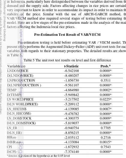
Based on literature review chapter before, according to Timmer (2008) Indonesia’s local rice price changes can be affected by a variety of factors such as paddy production, domestic stock, temperature changes, world prices, exchange rates, interest rates, and household consumption. In this section, we discussed about the models developed to explain the factors that affect the change in the price of rice in Indonesia, particularly here distinguished between the variables derived from the demand and the supply side. Factors affecting changes in rice prices are certainly very important to know in order to accommodate its impact in order to maintain the stability of the price. Similar with the use of ARCH-GARCH method, the VAR/VECM method also required several stages of testing before estimating the model. Here are a few stages of the pre-estimation made in the analysis of the main factors affecting the Indonesia local rice prices.
Pre-Estimation Test Result of VAR/VECM
Pra-estimation testing is held before estimating VAR / VECM model. The present study performs the Augmented Dickey–Fuller (ADF) unit root tests for each variables with regards to their stationary properties. The detailed results are shown in Table 5.
Table 5 The unit root test results on level and first difference
*denotes rejection of the hypothesis at the 0.05 level
Based on the unit root test result showed that LNPRODUCTION, CPI, LNER, and BIRate variables are not stationary in levels. Thus, unit root test is then
Variable (s) t-Statistic Prob.*
LNDOMRICE -6.542168 0.0000*
D(LNDOMRICE) -8.480207 0.0000*
LNPRODUCTION -1.856730 0.3511
D(LNPRODUCTION ) -9.561107 0.0000*
TEMP -4.664980 0.0002*
D(TEMP) -5.949842 0.0000*
LN WORLDPRICE -3.217502 0.0225*
D(LN WORLDPRICE) -5.209112 0.0000*
LN_HHCONS -4.139085 0.0087*
D(LN_HHCONS) -9.476782 0.0000*
LN_DOMSTOCK -4.300375 0.0009*
D(LN_DOMSTOCK) -5.819657 0.0000*
LN_ER -0.940754 0.7705
D(LN_ER) -8.856215 0.0000*
BIRate -2.035112 0.2716
D(BIRate) -4.133084 0.0015*
CPI -1.672932 0.7543
25 performed on the first difference with the results all of the variables were stationary on the significance level 5%. Further detail can be seen in Appendix 6.
While testing of VAR stability showed that all the roots polynomial function has a value of less than 1, with modulus value range from 0.09 – 0.99. This means that this VAR model are valid and stable so that the further analysis which is Impulse Response Function Analysis (IRF) and Forecast Error Decomposition (FEVD) are considered valid (See Appendix 7). The next step is the optimum lag testing based on SC (Schwartz Information Criterion). The minimum value showed that the optimum models is in lag 1. Further detail can be seen in Appendix 8.
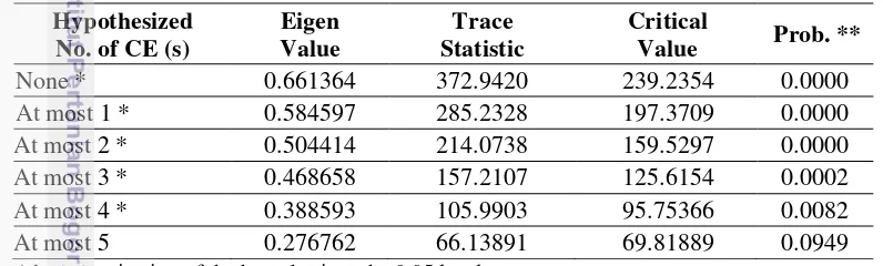
Testing cointegration is one of the important tests to be done when investigating the long-term relationship variables used in this study. Although the data used in this study is found individually not stationary, but it turns out that as a linear combination it becames stationary. One of the condition to achieved the long term balance (co-integrating) is the error value balance should fluctuate around zero. On the last stationarity testing before, noted that the variables used mostly stationary on a first difference. Thus if we were to used VECM estimation model, we should doing the cointegration testing first. The co-integration relationship in this study can be viewed from the statistic-trace value. If there is a cointegration, then the value of the trace statistic is greater than the value of the critical value 5 percent. This study using Johansen Cointegrating test. Following table are the result for each model.
Table 6 Johansen Cointegration test results
*denotes rejection of the hypothesis at the 0.05 level **MacKinnon-Haug-Michelis (1999) p-values
Table 6 shows that the model has trace-statistic value greater than the critical value 5 percent. Based on the trace test, the model indicates at most 4 cointegrating equation at 0.05 level (5% level). So, it can be concluded that for models of factors affecting rice price fluctuation, there is at least one cointegrating eqations which is able to explain the relationship between each variables in this model.
Factors Affecting Rice Price Fluctuation in Indonesia
Rice is one of the staple food commodities for the Indonesian people, where the fulfillment of rice in Indonesia should always be maintained at an affordable and stable price for the society welfare purpose. Thus, the stability of rice prices is important to keep. In order to maintain the stability of the domestic rice price, the government needs to find out what factors capable of influencing the fluctuating price of rice. By using VECM (Vector Error Correction Model), following are the result of variables that significantly affects the fluctuation of Indonesia local price in the short run and the long run.
26
Table 7 VECM estimation result
* significant for 5% level
t-critical value for 5% level is equal with 1.96
Based on Table 7, the local rice price, paddy production, domestic stock of rice, household comsumption, world rice price, temperature changes, exchange rate and interest rates play significant role in driving the rice price fluctuation in the long run. The Consumer Price Index (CPI) variables is the only variable that did not significantly affect the Indonesian rice price fluctuation.
In the long run, world rice prices have significant negative influence against domestic rice price changes amounted to 0.001. This coefficient means that if the world rice price increased by 1 percent, then the rice price volatility is likely to decrease by 0.001 percent. The explanation of this result can be seen from the Figure 6 and Figure 7 before, when the world rice prices has increased on the early 2008 before, but it has no effects on Indonesia’s rice price condition. Eventhough Indonesia act as one of the importing-rice countries, but this country seems not really get affected by the increasing price since the fulfillment of domestic needs of rice is still mainly contributed by domestic paddy production. Therefore changes in world rice price in the long rung has negatively affect the fluctuation of Indonesian domestic rice price.
Short-Run
Variable(s) Coefficient t-statistic value
D(VOLAT(-1)) -0.427258 -4.29702*
D(LNDOMRICE(-1)) 0.023818 5.25524*
D(LNPRODUCTION(-1)) 0.000311 1.33745
D(LN_DOMSTOCK(-1)) 0.001219 2.31668*
D(LN_HHCONS(-1)) 0.015416 1.37305
D(LNWORLDRICE(-1)) -0.000781 -0.87511
D(TEMP(-1)) 0.000698 3.38227*
D(LNER(-1)) -0.000636 -0.37713
D(BIRATE(-1)) 4.83E-05 0.11451
D(CPI(-1)) 4.75E-05 0.36970
Long Run
Variable(s) Coefficient t-statistic value
VOLAT(-1) 1.000000 -
LNDOMRICE(-1) 0.011034 4.76421*
LNPRODUCTION(-1) 0.002362 8.10346*
LN_DOMSTOCK(-1) 0.000979 2.32314*
LN_HHCONS(-1) -0.023510 -2.72450*
LNWORLDRICE(-1) 0.001804 2.94374*
TEMP(-1) -0.000277 -2.16775*
LNER(-1) 0.007229 3.43041*
BIRATE(-1) -0.000495 -2.14464*