5 CHAPTER 2
LITERATURE REVIEW AND THEORITICAL BACKGROUND
2.1. Literature Review
(Miller, Childers, and Taaffe 2009) conduct a research project to determine the
appropriate order quantity and forecasting methods for a local company
maintenances, repairs and overhaul inventory. According to their simulation
results, basing reorder quantities on the distribution of demand and accurate lead
time data showed significant improvement to the fill rate. They believe by
preventing stockouts will save a significant amount of money accross the
inventory system.
The research that is conducted by (Suryani 2012) is about analysis of the product
inventory control using genetic algorithm to minimize inventory cost. This
research at PT.XYZ who order the raw material A to the third parties by estimate
when the number of item in the warehouse is almost eshausted. When the
demand for item A againts PT.XYZ soaring frequently PT.XYZ can not meet the
demand. In other times PT.XYZ also have excess number of ordering goods, this
create an enormous amount of inventory that must be stored in warehouse, it can
affect the over runs of inventory cost.
Research conducted by (Chandra and Kumar 2006) is about the development of
the rules of new heuristic ordering multi item , single vendor inventory system
with random request. The position of the inventory for each item is a continuous
review and each message is when all stockout cost that projected to all aitem is
exceed certain multiple of the average fees.
Research that conducted by (Kao and Hsu 2002) is talk about lot size – reorder point inventory model with fuzzy demand. The objective is to find the best
inventory policy. The main problem in this research is in the inventory problem that has fuzzy demands. Methods that used are Yager’s Rangking method and five pair of simultaneous nonlinear equations. The results of this research by
using Yager’s ranking method can utilized to find the minimal total cost.
The other research was conducted by Pattnaik in 2012. This research is about
the constant demand model with the easy damage product whitin a certain
6
time. The objective of this research is to obtained the total cost of the damage
product such as fruits, vegetables and other kind of foods.
In 2010, Routroy and Bhausaheb conduct a research which is used simulation
with arena and the objective is to evaluate the inventory system for the damage
productd. The main problems on controlling the inventory of damage product are
the production cycle, order cost, holding cost, lost cost, overload cost, uncertainty
demand and the price of the products.
In actual inventory system, however multi-item storage is an issue typically
encountered. One research that formulated a novel approach for multi-product,
multi-period (Q,r) inventory models, with the objective of maximizing the profit
under constraints such as storage area, budget, shelf life, and various promotions
(Saracoglu, Topaloglu, and Keskinturk 2014). As the number of products and
periods increase, it can be found that an optimal solution cannot be reached with
ILP in a reasonable computational time. For this reason, we proposed a GA
solution approach since the problem of the pharmaceutical distributor case
studied is a larger sized problem.
Perbawa and Wigati (2014) analyzed the multi item inventory with demand and
probabilistic leadtime and limited warehouse capacity. The aim of this research is
to know when time to order the item and how much the quantity to obtain the
minimum total cost and there are no stockout in the warehouse while the capacity
is limited.
2.2. Theoretical Background
This section explains the theories that will be used in this research.
2.2.1. Definition of Inventory
Some inventories are in the form of raw materials and purchased item to be used
in making products, some are supplies to be used up in the manufacturing
process, some are partially manufactured items (work in process) in prodution
departments, some are finished parts ready to be put into assembled products,
some are finished products in shipping rooms and warehouses (Moore and
Hendrick, 1980: 334). In other hand, inventory is defined as goods that are stored
for use or sale in the future (Kusuma, 2004:131). Inventory is the important thing
7
Inventories make possible a rational production system. Without inventory
company could not achieve smooth production flow. An inventory is a list of the
items held in stock (Waters, 2003:3). Operation manager in the entire world
reliazed that the good inventory management is so important. In the other side, a
company can decrease the cost by decreasing the inventory. The production also
can be stop and the costumer feel disappointed if the order is not available
(Heizer & Render,2014:553).
2.2.2. Stoks Cycles
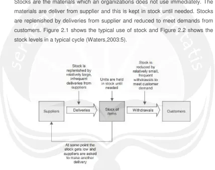
Stocks are the materials which an organizations does not use immediately. The
materials are deliver from supplier and this is kept in stock until needed. Stocks
are replenished by deliveries from supplier and reduced to meet demands from
customers. Figure 2.1 shows the typical use of stock and Figure 2.2 shows the
stock levels in a typical cycle (Waters,2003:5).
Figure 2.1 The Typical Use of Stock. Source: (Waters,2003)
Typically, each cycle has the following elements such as:
a. An organizations buys a number of units of an item from a supplier
b. At an arranged time, these units are delivered
c. Unless they are needed immediately, the units are put into storage,
replenishing the stocks
8
e. Unit are removed from stock to meet these demand
f. At some point, the stock obtains low and it is time for the organization to place
another order.
Figure 2.2 Stock Levels in a Typical Cycle Source: (Waters,2003)
Usually, deliveries from supplier are relatively large and infrequent, while
demands from customer are smaller and more numerous, giving the typical
pattern. The main purpose of stocks is to give a buffer between supply and
demand.
2.2.3. Types of Inventory
The organizations has different types of stock or inventory. A useful classification
has (Waters, 2003:9):
a. Raw material, which have arrived from supplier and kept until needed for
operations.
b. Work in progress, which are units currently being worked on
c. Finished goods, which are waiting to be shipped to customers.
9
e. Consumable, such as oil, paper, cleaners, etc.
Raw material inventory has been purchased but not process yet. This kind of
inventory can be used to seperates supplier from the production process.
Nevertheless, a preferred approach is to remove the variability of suppliers in
quality, quantity or delivery time so that there are no need to be separated(Heizer
& Render,2014:554). The example for raw material are woods, fabrics and so on
waiting to be made into articles. Work in progress inventory is components or raw
materials that has passed through several processes of change, but not complete
yet. There are work in process to make an product needs time (cycle time).
Decrease the cycle time also will decrease the work in process inventory (Heizer
& Render,2014:554). The example of work in process is the articles being worked
on at the moment. Finishied good inventory is the finished product and already to
be delivered. The finished good can be entered into the inventory because
customer demand in the future is unknown(Heizer & Render,2014:554). The
example of finished goods are articles waiting to be delivered to the customers.
The example of inventory spare parts are kept for the knitting machines and other
equipment and for consumable inventory include cleaners, stationery and other
material to keep operations going.
2.2.4. Function of Inventory
Planning and inventory control is useful to make a stable condition for the
production process and marketing. The aim of stock the raw material is to
reducing production uncertainty due to raw material fluctuations. Inventory can have a variety of functions that add to the flexibility of the company’s operations. There are four function of inventory (Heizer & Render,2014:553) :
a. To provides a large selection of goods in order to meet anticipated customer
demand and separates the company from fluctuations in demand. This kind of
inventory generaly uses for retail company.
b. To separates the multiple stages of the production process. For example, if a
company inventory fluctuates, additional inventories may be required in order
to separate the production process of the supplier.
c. To takes advantage of a number of pieces for large purchases can decrease
the cost of delivery the goods.
10 2.2.5. Inventory Cost
All stocks incur costs. Therefore the organizations want to minimize the inventory
cost but the organization can not reducing the stocks. Actually low cost give a
minimum cost, but low stock can lead to shortages. The usual approach
describes four types of cost such as (Waters, 2003:52) :
a. Unit Cost
This is the price charged by suppliers for one unit of the item or the cost to the
organization of acquiring one unit. In general, it is fairly easy to find values for
the unit cost by looking at quotations or recent invoices from suppliers.
b. Reorder Cost
This is the cost of placing a repeat order for the item and mightinclude
allowances for drawing-up an order (with checking, obtaining authorization,
clearance and distribution), correspondence and telephone costs, receiving
(with unloading, checking and testing), supervision, use of equipment and
follow-up. Sometimes costs such as quality control, transport, delivery, sorting
and movement of received goods are included in the reorder cost.
c. Holding Cost
Holding many stock is expensive. This is the cost of holding one unit of an
item in stock for one period of time. The most obvious cost of holding stock is
money tied up- which is either borrowed (in which case there is interest to
pay), or could be put to other use(in which case there are opportunity costs).
Other holding costs are due to storage space(supplying a warehouse, rent,
rates, heat, light, etc), loss(due to damage, obsolescence and pilferage),
handling (including all movement, special packaging, refrigerator, putting on
pallets, etc), administration (stock checks, computer updates, etc) and
insurance.
d. Shortage Cost
If an organization runs out of stock for an item and there is demand from a
customer, then there is a shortage that has an associated cost. Any
shortage of parts for production might cause considerable disruption and force
emergency procedures, rescheduling of operations, retiming of maintenance
period, laying-off employees, and so on.
2.2.7. Probabilistic Inventory
There is uncertainty in almost all inventory systems. Some of this is under the
11
reliability (Waters,2003:152). Probabilistic models can be used when the demand
of product is unknown but can be determined by using probability distribution. An
probabilistic model is the adjustment in the real world because of the demand
and the waiting time is not always known and it is constant (Heizer &
Render,2014:575). The unconstant demand can increase the probability of
inventory stockout.
2.2.8. Definition of Simulation
Simulation is based on an appropriate model. Simulation gives a dynamic
representation of a real operations (Waters, 2003). A simulation model is
however in principle associated with the same limitations as all other
mathematical models. A simulation model can never give a complete illustration
of the real system. Note especially that if a simulation model is based on the
same assumption as some other inventory model the result will of course be the
same and simulations will therefore not give any additional insight. Simulation
can give valuable information, though if the simulation model illustrates the real
system better in some way. Assume, for example that the determination of safety
stocks in an inventory control system is based on the assumption of a certain
demand distribution and that it has not been possible to analition. A simulation
model based on real historiical demand data can then be used for analyzing
whether the demand distribution used is reasonable (Axsater,2000:182).
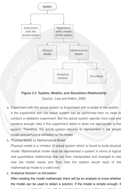
2.2.9. System, Models and Simulations
A great simulation is determined by resulting the great model. While the great
model will be resulted through a great observation for the system. Figure 2.3.
12 System
Experiment with the actual system
Experiment with a model of the system
Physical Model
Mathematical Model
Analytical
Solution Simulation
Figure 2.3. System, Models, and Simulation Relationship Source : Law and Kelton, 2000
a. Experiment with the actual system vs Experiment with a model of the system
If the experiment with the actual system can be performed then no need to
conduct a validation experiment. But the actual system spends more cost and
contains enough risks if this experiment failed or does not appropriate to the
system. Therefore, the actual system requires to represented in the simple
model and perform a validation to the model.
b. Physical Model vs Mathematical Model
Physical model is a miniatur of actual system which is found to build physical
model. Mathematical model must be represented a system in terms of logical
and quantitative relationship that are then manipulated and changed to see
how the model reacts and thus how the system would react (if the
mathematical model is a valid one)
c. Analytical Solution vs Simulation
After creating the model mathematic there will be an analysis to know whether
the model can be used to obtain a solution. If the model is simple enough, it
13
exact, analytical solution. But for the complex model, the mathematical model
is difficult to perform using analytical solution and needs more time, so that
simulation can be performed to obtain the solution from the complex system.
2.2.10 Advantage and Disadvantage of Simulation
Simulation is a familiar method that used to solved the complex problem.
Therefore, the following is advantages of simulation according to Law & Kelton
(2000).
a. System in the real life is very complex. Therefore there can not be described
accuratly with the mathematical model which can be evaluated in analitic. So ,
simulation is common to use to analyse the problem.
b. Simulation is possible to performance estimation from the system which is in
the setting operation condition that projected.
c. The design of alternative system that proposed can be compared through
simulation to know which alternative that fulfill the criteria that needed.
d. Through the simulation, in controlling the experiment condition can be kept
better than its system.
e. Simulation is possible to conduct the research in long term.
While that, simulation also has disadavantages. This following shows the
disadvantages of simulation.
a. Simulation model just resulting the estimation value from inputed parameter.
b. If the model is not represent the validation of system then the result of
simulation only to give an information about the real system.
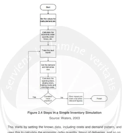
2.2.11. Simulation Steps
In conducting the simulation, there are some steps that must be done. Simulation’s steps not only straight to the next step but also can go back to the base steps. The first step in building a simulation model is to describe the
operations in detail. There are several ways of doing this, with the most common
using a flow diagram show the sequence of activities. Figure 2.4 shows the steps
14
Figure 2.4 Steps in a Simple Inventory Simulation Source: Waters, 2003
This starts by setting the known data, including costs and demand pattern, and
uses this to calculate the economic order quantity, timing of deliveries, and so on.
Then take the first month, check the demand and deliveries due, find the opening stock, set the opening stock (which is last month’s closing stock), find the closing stock(which is opening stock plus deliveries minus demand) and calculate all the
costs. Then go to the second month and repeat the analysis. This can continue
for as many repetitions as needed to obtain a longer-term view of the economic
order quantity. All the calculations for this are done with appropriate software.
That was the basic steps of simulation and can start by adding some more details
to give a better picture of the real system. For example, vary the pattern of
demand rather than consider one fixed pattern and add a variable lead time and
amount delivered(perhaps allowing for quality checks). The way of introducing
15
know exactly the demand in a month, but know that it is between 30 and 50 units.
The spreadsheets can automatically generate random values and in Microsoft
Excel the function RANDBETWEEN(30,50) will generate a random value
between 30 and 50. The random variations mean that each run will be different.
To find the real pattern we would have to repeat the simulation many times,
perhaps hundreds or even thousands (Waters, 2003: 294) .
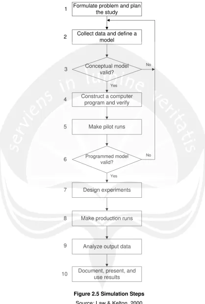
In another hand, (Law & Kelton, 2000) a simulation starts from formulate the
problem formulation. Then the next step is collecting the data and determine the
model according to the real problem. After the model had conducted then check
the model, is the model valid or not. If the model is invalid then conduct the
re-problem formulation. But if the model is valid then conduct the verification. After
all clear, then design the experiment such as determining the lead time, set up
time, and the number of replications. The next step is running the program and
conduct the data analysis. Analysis data was conducted to decide the system
and compare all available alternatives. After the output had already analyzed and
compared also got the result, the last steps is documenting the model that will be
uses for future and apply the simulation result. Figure 2.4 shows the simulation
16
Formulate problem and plan the study
Collect data and define a model
Construct a computer program and verify
Conceptual model valid?
Make pilot runs
Design experiments Programmed model
valid?
Make production runs
Analyze output data
Document, present, and use results
1
Yes
Yes
No No
2
9 8 7 6 5 4 3
10
17 2.2.12. Verification
Verification is used to decide whether the simulation model is already closed to
the real system or not. One of the technique is to conduct the verification by run
the simulation under the variety of setting the input parameters, then check
whether the output can be accepted or not (Law&Kelton, 2000).
2.2.13. Validation
Validation is a process of determining whether or not the simulation model is
already represent the real condition accurately. It is used to test the model and
compare to the real system. Validation is conducted by using one of tools in Ms.
Excel Software that is t-test: Two-sample assuming equal variances. This test is
assume that both of data is from the population with the same variances. The
validation test compares the real data with the data from simulation (Law &
Kelton, 2000). If there is no significantly different, then the model can be said as a
valid model.
2.2.14. Replication
To run the simulation it is not enough if there just once to represent the real
condition. Therefore the simulation needs to run more than once. Replication is
needed to determine how many simulations to run. Parameter that used to decide
the number of replication is the total end cost of inventory.
In determining the number of replication, first step are decide the coefiecient of
confidence interval (α) and level of error ( ). The value of α that used is 0.1 that is
mean there is an possible of 0.1 for the value of mean will out of the range ̅
. The value of coeficient is 0.1 which means the value of deviation of ̅ from. The value of can be obtained with this following formula (Law and
Kelton, 2000)
| ̅̅̅̅̅̅| (2.1)
| | | | (2.2.)
After that, the number of replication can be obtained when the condition achieved
18
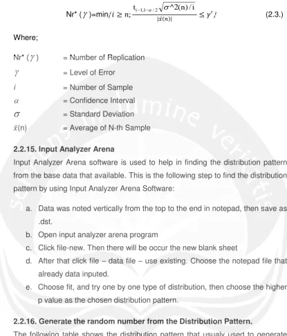
Nr* (
)=min ti1,1/2 ^2(n)/i| ̅ | (2.3.)
Where;
Nr* (
) = Number of Replication
= Level of Errori = Number of Sample
= Confidence Interval
= Standard Deviation ̅(n) = Average of N-th Sample2.2.15. Input Analyzer Arena
Input Analyzer Arena software is used to help in finding the distribution pattern
from the base data that available. This is the following step to find the distribution
pattern by using Input Analyzer Arena Software:
a. Data was noted vertically from the top to the end in notepad, then save as
.dst.
b. Open input analyzer arena program
c. Click file-new. Then there will be occur the new blank sheet
d. After that click file – data file – use existing. Choose the notepad file that
already data inputed.
e. Choose fit, and try one by one type of distribution, then choose the higher
p value as the chosen distribution pattern.
2.2.16. Generate the random number from the Distribution Pattern.
The following table shows the distribution pattern that usualy used to generate
the random number in simulation using Microsoft Excel (Law and Kelton, 2000).
Table 2.1. Generate Distribution Pattern in Microsoft Excel
Name Distribution X
Uniform UNIF (Min, Max) Min + (Max-Min). U
Exponential EXPO (µ) - µ . ln(U)
Weibull WEIB ( , α) [-ln(U)].1/ α
Gamma GAMM ( , α) GAMMAINV(U; ; α)
19
X = The result of generated random value
U = Random value, 0 ≤ U ≤ 1
2.2.17. Half Width, Upper and Lower Confidence Interval
Half width is the confidence interval which has exact interval in the confidence
level to the real average value (Law and Kelton, 2000).