Statistical power analysis for one way a

(1)

Statistical power analysis for one-way

analysis of variance: A computer program

Article in Behavior Research Methods · May 1990

DOI: 10.3758/BF03209816

CITATIONS

18

READS

52

5 authors, including:

Michael Borenstein

Biostadt

90PUBLICATIONS 7,780CITATIONS

SEE PROFILE

Hannah Rothstein

City University of New York - Bernard M. …

64PUBLICATIONS 6,038CITATIONS

SEE PROFILE

All content following this page was uploaded by Hannah Rothstein on 05 February 2014.

(2)

-

METHODS & DESIGNS

Statistical power analysis for one-way analysis

of variance: A computer program

MICHAEL BORENSTEIN

Hillside Hospital, Long Island Jewish Medical Center, Glen Oaks, New York and Biostatistical Programming Associates, Teaneck, New Jersey

JACOB COHEN

Biostatistical Programming Associates, Teaneck, New Jersey and New York University, New York, New York

HANNAHR. ROTHSTEIN

Baruch College, City University of New York, New York, New York

SIMCHA POLLACK

Hillside Hospital, Long Island Jewish Medical Center, Glen Oaks, New York Biostatistical Programming Associates, Teaneck, New Jersey

and St. Johns University, Jamaica, New York and

JOHN M. KANE

Hillside Hospital, Long Island Jewish Medical Center, Glen Oaks, New York

To facilitate the computation of statistical power for analysis of variance, Cohen developed the index of effect sizef,defined as theSDbetween groups divided by theSDwithin groups. A micro-computer program for statistical power allows the user to compute the value offinany of several ways: by specifying the mean and SDfor every cell in the ANOVA; by specifying the mean value for the two extreme cells and the pattern of dispersion for the remaining cells; by estimating the proportion of variance in the dependent variable that will be explained by group member-ship; and/or with reference to conventions for small, medium, and large effects. The program will compute power for any single set of parameters; it will also allow the user to generate tables and graphs showing how power will vary as a function of effect size, sample size, and ex.

The process of statistical inference carries with it the potential for two types of error: A Type I error, which is made when the treatment under study is actually not effective but the researcher concludes that it is effective, and a Type IIerror, which is made when the treatment actually is effective but the researcher concludes that it isnot.

The probability that the study will result in a TypeII

error ({3); or, expressed conversely, the probability that the study will yield significant results if the treatment is effective (the study's power) is a function of three fac-tors:(1) sample size (the higher the sample size, the more

This research was supported in part by the following grants: NIMH/SBIR l-R43-MH-43083-Ql, NIMH/SBIR l-R43-MH-43083-02, and NIMH MH-41960-02. The authors would also like to express their appreciation to the editor and reviewers for their comments on an earlier draft of this paper. Correspondence should be addressed to Michael Borenstein, Hillside Hospital, A Division of Long Island Jewish Medical Center, P.O.B. 38, Glen Oaks, NY 11004.

confidence we have in the observed effect and so the higher the power); (2) c<(the more liberal the criterion that will be accepted as valid, the higher the power); and(3)effect size (the larger the population effect, the more likely that the effect observed in the study will meet the criterion for statistical significance, and the higher the power).

Itfollows that in order to compute power, the researcher must provide an estimate of the hypothesized effect size. Whereas the specification of an effect size is fairly direct forttests (typically, the standardized mean difference is

used, as in Dunlap, 1981), for correlations (the correla-tion coefficient itself serves as the effect size, asinDunlap

& Kemery, 1985), or proportions (the proportion ofposi-tive cases in each group is reported, as in Dunlap, 1982), the specification of an effect size for analysis of variance or covariance is problematic, since the effect is a function of the dispersion among and within any number of groups. One index of effect size that can be applied to analysis of variance is the noncentrality parameter¢(Odeh& Fox, 1975), and computer programs that compute power for

(3)

analysis of variance typically require the user to specify the effect size as some variant of this parameter (see Goldstein, 1989).This approach is less than ideal, how-ever, since ¢ is determined not only by the effect size but also by the sample size. For the purpose of power analysis, it would be preferable to use an index that was determined solely by the magnitude of the effect, so that the researcher could develop an intuitive feel for the in-dex, and could manipulate the effect size and the sample size independently of each other.

This need for a standardized measure of effect size is addressed by the index

f

developed by Cohen(1977, 1988;

Borenstein & Cohen, 1988). In the present paper, we describe this index and present a computer program that enables the researcher to computef, and, usingf, to de-termine power for analysis of variance or covariance.

The

f

Index of Effect Size

To facilitate computation of power, Cohen(1977, 1988)

suggested the use of an effect size index,j, defined as the ratioSDBetween Groups/SDWithin Groups(i.e., SDB/SDw)-which is not to be confused with the test statistic denoted by an uppercaseF.Intheory, this index can range in value from zero to an indefinitely high positive value, but in practice, it typically falls in the range from zero (indicat-ing no effect; i.e.,the null hypothesis) to0.40 (represent-ing an effect that is larger than is typically found in so-cial science research). Since researchers are not generally familiar withf, it would be instructive to place this index in the context of other indices of effect size.

The effect size

f

in relation to effect size d. Cohen

(1977, 1988)created the indexdas a measure of effect size for the difference between two group means that are to be compared by a ttest. This index is defined as the

standardized mean difference(i.e.,the absolute value of the mean difference divided by the standard deviation within a group). The indexfmay be seen as the extension of this concept to the case of multiple group means and analysis of variance, in thatfis again the standardized mea-sure of dispersion between groups; but in this case, dis-persion among multiple groups is defined in terms of the assumed (population) standard deviation between groups rather than in terms of the (population) difference score. When the analysis is limited to two groups, the re-searcher has the option of comparing the groups byttest

and applying the effect sized,or of comparing the groups by analysis of variance and applying the effect size

f

In this case,dandfare related by the functionf

=

d/2.For example, if we posit means of10versus 15,and SDw of10,dwould be equal to(15-10)/10, or0.5. Equiva-lently, fwould equal 2.5/10, or 0.25.

When there are more than two groups, the correspon-dence betweend and

f

is more complex, since d is able to account for only two means, whereas

f

incorporates information about more than two means. In this case, d may be calculated on the basis of the single lowest and highest group means, adjusted to reflect the dispersion of the additional group means, and then used to derive a value forf. The dispersion of the group means may be

described as matching one of three patterns, as follows:

(1)The remaining groups fall at the midpoint between the two extreme groups; this serves to minimize the between-groups dispersion and yields the lowest valueoff.(2) The remaining groups are spread evenly over the entire range between the two extremes; this results in somewhat more dispersion between groups than in the previous case, and a somewhat higher value forf. (3) The remaining groups fall at either extreme; this results in the highest possible dispersion between groups and the highest valueoff,given the constraints imposed by the two extreme means and theSD.The precise function for calculating fin this man-ner is presented in Appendix A.

The effect size

f

inrelation to ."1. An intuitive mea-sure of effect size, ."1is defined as the proportion of vari-ance in the dependent variable that may be explained as a function of group membership.

.,,1

is thus the ANOVA analogue toR1,the value that would be cited in the case of multiple regression. The effect size

f

is related to ."1 by the function

f=

-JP

where

.,,1

I'

=

-I- 1 '

-."

In the range of.,,2 typically encountered (0.0-0.14),

f2will be roughly comparable to.,,2, andfwill be roughly comparable to the correlation coefficient r.

linrelation to

cp.

The index

cp,

which is used in other treatments of power (see, e.g., Odeh&Fox, 1975;Owen,

1962; Scheffe, 1959; Winer, 1971), standardizes the magnitude of the effect by the standard error of the sam-ple mean and is thus (in part) a function of the size of each sample,

n,

whilefis solely a descriptor of the

popu-lation (Cohen, 1988).The relationship betweenfand ¢ is given by

¢ f=

--In

or

¢

=

f-Jn.

(4)

TheSD Bis 2.5 units and the SDw is 25 units;

f

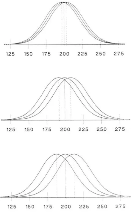
would be calculated asSD B/SDw(2.5/25), or 0.10. This mag-nitude of effect is displayed in the top segment of Fig-ure 1.

A medium effect (f= .25) corresponds to the case in which the between-groups dispersion is one fourth as large as the within-groups dispersion. Equivalently,

f

= .25 in-dicates that some 6% of the variance in the dependent vari-able is explained by group membership. To extend the cholesterol example, the same researcher is thinking about comparing the cholesterol levels of three groups that report no exercise, minimal exercise, and moderate ex-ercise, respectively. In this case, the researcher believes that the group means will vary over 16 units (192, 200, 208). The SD Bis 6.5 units and the SDwis 25 units;

f

would be calculated asSDB/SDw(6.5/25), or 0.24. This effect is shown in the middle segment of Figure 1.

A large effect(f

=

.40) indicates that theSDBis four

tenths as large as theSDw .Equivalently, it implies that

14% of the variance in the dependent variable may be

ex-125 150 175 200 225 250 275

125 150 175 200 225 250 275

Figure 1.This figure displays three hypothetical studies. The top segment represents asmalleffect size(j

=

.10); the middle segment represents a medium effectsize(j"" 0.25); and the bottom segment represents a large effect size (/ "" 0.40). In each case, the means of the three distributions are indicated by vertical lines.

plained by group membership. In the running example, the researcher is thinking about comparing the cholesterol levels in three groups whose diets differ in more substan-tial ways (i.e., a group of people who avoid foods high in cholesterol, a group that eats these foods in modera-tion, and a group that eats them on a regular basis). The researcher believes that the mean cholesterol levels for these groups will range over 24 units (188, 200, 212). The SDBis 9.75 units and theSDwis 25 units;fwould be calculated asSDB/SD w (9.75/25), or 0.39. This ef-fect is shown in the bottom segment of Figure 1.

Use of the index

f

in analysis of covariance. The preceding discussionoffas an index for analysis of vari-ance may be applied to analysis of covarivari-ance as well, except that in this case the dependent variable of interest is now adjusted to take account of the covariate. Con-cretely, the formula SDB/SDw now applies to theSDs of theadjustedmeans. Typically, the denominator will shrink (the adjusted SDw is equal to the original SDw, multiplied by

-J

I -

r.h

where X is the covariate andYis the dependent variable), while the numerator will undergo no systematic change (and may increase). Therefore, the effective

f

for analysis of covariance will be greater than the

f

for the corresponding ANOVA. Equivalently, if

f

is conceptualized in relation to the effect indexd, theSD used in computingdwould be reduced with a correspond-ing increase indand

f

Finally, iffis perceived in terms of the proportion of variance explained, the total variance to be explained is now reduced by the use of a covariate: The amount of variance explained by group membership is now seen as a proportion, not of the whole, but of the part that remains unexplained following the introduction of the covariate. A more detailed discussion of these points is provided in Cohen (1988).

In the balance of this paper, we describe a computer pro-gram that enables the user to compute power for analysis of variance or covariance, by specifying the effect size fwith reference to any of the definitions discussed above.

Operation of the Program

Overview. The user is presented with a spreadsheet (Figure 2) and prompted to enter values for the total sam-ple size(N), the number of cells in the one-way ANOVA

(k), a, and the effect size

f

The cursor keys allow the user to move freely between cells and repeatedly modify any value(s) without having to reenter the other values. Afterallvalues have been entered or modified in this way, the user presses

<

F9

>

and the program reports the value of power.

HELP screens for calculating

f.

While any of the re-quired values may be entered directly, the user will typi-cally require some assistance in determining an appropri-ate value for the index

f

For this reason, the program incorporates various HELP screens that enable the user to compute

f

by entering the individual cell means and SDs;to derive a value for fbased on its association with d or T/2;or to assign a value based on the conventions [image:4.558.50.270.305.662.2]

(5)

Cursor <UP><DOWN> <LEFT><RIGHT> to Locate a Value Press <ESC> or <BACKSPACE> to Erase that Value

Then use the TOP ROW of the keyboard to enter the new value

<F9> PROCEED WITH COMPUTATIONS <FlO> EXIT

Effect size f TOTAL N

Number of Groups Alpha

Enter the Effect Size f, or

<F3> Enter Value for each cell <F5> Enter Proportion variance

0.280 80

4

0.050

[image:5.558.48.514.58.346.2]

<Fl> General HELP Screen <F4> Enter Range of cells <F6> view/Modify in Context

Figure 2. The user enters values forN,number of groups, andQ.The effect sizef mayalsobe entered directly from this screen.

Alter-natively, tbe user may invoke oneoftbe otber screens and allow tbeprogram to computef.

Cursor <UP><DOWN> <LEFT><RIGHT> to Locate a Value Press <ESC> or <BACKSPACE> to Erase that Value

Then use the TOP ROW of the keyboard to enter the new value

<F9> COMPUTE f <FlO> EXIT TO PROGRAM WITHOUT COMPUTING f

MEAN STD DEV N

Group # 1 45.000 20.000 20

Group # 2 50.000 20.000 20

Group # 3 55.000 20.000 20

Group # 4 60.000 20.000 20

VALUE OF f= 0.28 TOTAL N= 80 MEAN N PER CELL: 20

Press <SPACE> to make additional modifications on this screen

Press < F9 > to transfer value of f and N-Cases to program

Press < FlO > to return to program without transferring values

[image:5.558.48.515.415.698.2]

(6)

the computational algorithms are presented in Ap-pendix A.

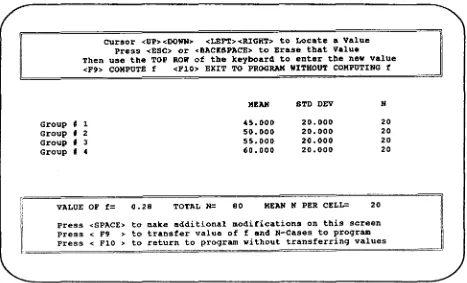
Method 1: Exact calculation offBy pressing

<

F3

> ,

the user transfers control of the program to the HELP screen shown in Figure 3, and is asked to enter the mean, SD,andn for every cell in the ANOVA. When the user presses

<

F9

> ,

the program calculatesfby the formula SDB/SDwand transfers this value to the main program.

Method2:Approximate calculation off based on ex-treme cells and pattern ofdispersion. In some cases, the user will find it difficult to specify a mean for each cell in the ANOVA, but will have a fairly accurate idea of the means for the extreme cells. By pressing

<

F4

> ,

the user invokes the HELP screen shown in Figure 4, and is asked to enter the mean for the two extreme cells, the SDwithin cells, and the pattern of dispersion for the re-maining cells (clustered at the center, evenly spaced, or clustered at the extremes). The user then presses

<

F9

>

to compute the approximate value of

f

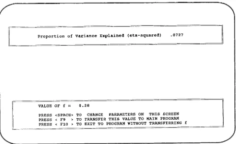
and transfer this value to the main program.

Method3:Calculation offas a function of7j2. By press-ing

<

F5

> ,

the user invokesthe screen shown in Figure 5. The program reports that the

f

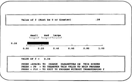
value specified earlier would correspond to7/2of 0.07, indicating that some 7% of the variance in the dependent variable is accounted for by group membership. The user may accept this value and return to the main screen. Alternatively, the user may elect to type in a new value for 7j2. In this case the pro-gram would compute the corresponding value off, and then transfer this value to the main program.

Method 4:Specifyingfin the context ofsmall, medium, and large effect sizes.Bypressing

<

F6

> ,

the user invokes a screen in which the most recently specified valueoff

is displayed as a bar graph on which the points correspond-ing to small, medium, and large effects are highlighted (Figure 6). Thus, the user is able to satisfy himself or her-self that the specifications entered by one of the other methods are consistent with the magnitude of effect that is typical in the given field of study. The user has the op-tion of entering a new value for

f

on the basis of the dis-played conventions, and then transferring this value to the main program.

Putting it all in perspective. Thus, the valueoffmay be entered directly into the main program or calculated via any of these HELP screens. The user who is able to specify a mean and anSDfor every cell in the ANOVA would want to use the first method to calculate an exact value for

f

The user who is not able to specify a value for every cell, but is able to estimate the value of the two extreme means, theSDwithin cells, and the pattern for the other cells, would use the second method to derive an estimate for

f

The third method involves no assump-tions about the means orSDof any cell. In this case, the user is required only to specify the proportion of vari-ance in the dependent variable that will be explained by group membership. The final method requires simply that the user choose a value based on conventions.

These various HELP screens are linked to each other, so that the user may calculate and view the valueoffin

any number of ways, to ensure that the value selected is appropriate from more than one perspective. For exam-ple, the user might calculate

f

initially by Method I, specifying the mean, SD,andn for every cell as shown in Figure 3, and findingthatf= 0.28. Alternatively, the user might calculate

f

initially by Method 2, providing the values for extreme means shown in Figure 4 and find-ing thatf= .28. (Note that the values in these two figures

describe the same population, and that both methods yield the same value forf). Whether the initial estimate of

f

had been obtained by the first or the second method, the user might then proceed to invoke Method 3, and observe that anfvalue of 0.28 corresponds to7/ 2of 0.07, indicat-ing that 7% of the variance in the dependent variable may be explained by group membership. Finally, the user might invoke Method 4, and note that the specified effect

off

=

.28 places this effect slightly above the value (0.25) adopted as a medium effect size (Figure 6).Ifthese values are consistent with the user's expectations, he or she would proceed to compute power. Otherwise, the user would be free to modify the specified effect size at any point.

Program Options

Calculation of power for a single set of parameters. After providing values for sample size, number of groups, a, and the effect size

I.

the user may press

<

F9

>

to dis-play the corresponding value of power.

Tables of power as a function of effect sizeand sam-ple size. The user who is planning a study will typically want to know how power varies as modifications are made to the effect size (what happens if the population effect is actually smaller or larger than our projections?) and sample size (how much would power increase if the sam-ple size were increased byNsubjects?). The program al-lows the user to specify up to four values for

f

and up to 70 values for sample size (e.g. ,jvaries from 0.10 by 0.10 to 0.40, andNvaries from 20 by 2 to 150). The pro-gram will then create a table (Figure 7) that shows power as a function of these values. In this example, the status lines at the top of the screen indicate that the number of groups is constant at 4 and thatais constant at 0.05, while

f

and Nare allowed to vary. Ifwe assume an effect of

f

=

.30 and want to work with power of 0.80, the study would require a total of 124 subjects divided among the four groups.

(7)

4

J

20

45

----J

60

2

=:J

I

CLUSTERED

I

SPACED EVENLY

III

EXTREME

III

IIIII

Mean for the LOWEST group in study Mean for the HIGHEST group in study

Pattern for all groups <Fl for Help> Number of Groups

standard Deviation WITHIN a group

PATTERN 2 PATTERN 1

PATTERN 3

[ , , = = = = = = = = = = = =

｛ｾｾｾｾ］Ｇ

= = = = =

If

L-==========

VALUE OF f

=

0.28

PRESS <SPACE> TO CHANGE PARAMETERS ON THIS SCREEN

PRESS < F9 > TO TRANSFER THIS VALUE TO MAIN PROGRAM

[image:7.558.48.515.46.329.2]

PRESS < FlO > TO EXIT TO PROGRAM WITHOUT TRANSFERRING VALUE OF f

Figure 4. Method 2: The user specifiesthe mean for the lowestand the highest cells.Inaddition, the user reports the pattern of disper-sion for the remaining cells. (Pattern 1 includes five overlapping points at the center, and Pattern 3 includes three overlapping points at either extreme. On the two-dimensional screen, these overlapping points are displayed as adjacent to each other.) The program

esti-mates the corresponding value of

f.

.0727 Proportion of variance Explained (eta-squared)

ｬｾ］］］］］

VALUE OF f

=

0.28

PRESS < FlO > TO EXIT TO PROGRAM WITHOUT TRANSFERRING f

｟Ｎ｟Ｎｾ］］］］］］］］］］］］］］］］］］］］］］］］］ｾ

Figure 5. Method 3: This screen shows thef value computed earlier would imply that ,,'is0.07; that is, some 7% of the variance in the dependent variable may be explained by group membership. The user could elect to type in another value for ,,' at this point, and

[image:7.558.50.514.404.688.2]

(8)

Value ot t (Must be 0 or Greater) .28

]

Small Med Large

I I I I I

0.28

ｾ

0.00 0.20 0.40 0.60 0.80 1.00

VALUE OF t : 0.28

[image:8.558.47.512.50.339.2]

PRESS < FlO > TO EXIT TO PROGRAM WITHOUT TRANSFERRING t

Figure 6. Metbod 4:ThIsscreen shows that the/value computed earlier would correspond to a medium effect size.Theprogram allows

the user to modify the value of / from this screen as well.

f : VARIES GROUPS: 4

N TOT : VARIES ALPHA : 0.050

N TOT f : f : t : _f :

! 0.100 0.200 0.300 0.400

110 0.120 0.389 0.747 0.949

112 0.121 0.396 0.756 0.953

114 0.123 0.403 0.764 0.957

116 0.124 0.409 0.772 0.960

118 0.126 0.416 0.780 0.963

120 0.128 0.423 0.788 0.966

122 0.129 0.429 0.795 0.968

124 0.131 0.436 0.802 0.971

126 0.132 0.443 0.809 0.973

128 0.134 0.449 0.816 0.975

130 0.136 0.455 0.823 0.977

132 0.137 0.462 0.829 0.979

<4> DISPLAY LINE GRAPH <5> PRINT FULL TABLE < 6> PRINT SCREEN

CURSOR <UP> OR <DOWN> TO SCROLL TABLE <10> EXIT

(9)

f

=

N TOT

=

0.300124 GROUPS=ALPHA

=

0.0504 0.8024POWER= <l>HELP<3>TABLE

1.00

0.75

0.50

0.25

0.00

•••••••••••••••••

•••••••••••••••

...

ｾ

•••••

··1···

•••• • • • • • • • • t

••••

•••

••

•••

••

• ••••••• • • 0

••••••••••• 0000000000000000000000000000000000000000

·000000000000000000000000000

N TOT 20 34 48 62 76 90 104 118 132 146

Figure 8. This graph shows how power (on the vertical axis) will vary as a function of effect size (represented by the four lines) and sample size (on the horizontal axis). The cursor keys are usedto highlight any point on the graph, and precise values for that point are presented at the top of the screen.

Interface to other programs.The program allows the tables and graphs to be sent to the printer or to an ASCII file which may then be input into other programs for ad-ditional manipulations.

Algorithms

Power is calculated by determining the upper tail area of the noncentralFdistribution, corresponding to the al-ternate hypothesis, that exceeds the critical value for F under the null hypothesis. This approach relies on three algorithms. A subroutine adapted from equation 26.2.19 in Abramowitz and Stegun (1965) reports the value of z corresponding toa. This value, together with values for dfand effect size, is sent to a subroutine that uses the Laubscher (1960) chi-SQuare-based square root algorithm to approximate the noncentralFdistribution, and returns a value of z corresponding to power (see also Cohen &

Nee, 1987, and Fowler, 1984, for a discussion ofthis al-gorithm's accuracy). This z value is used to compute the area under the curve, or power, by means of the Odeh and Evans (1974) algorithm for approximation of the in-verse normal distribution function (see also Brophy, 1985). Additional details of the computational algorithms are given in Appendix B.

Accuracy

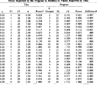
To assess the accuracy of the program, values gener-ated by the program were compared with the exact values reported by Tiku (1967), who used the method described

by Tang (1938). This comparison was carried out for a

=

.01, .05;dfnum

=

1, 3, 9 (corresponding to number of groups

=

2, 4, 10),dIerror

=

8, 10, 20, 40, 120; and cP(used by Tiku) corresponding to 0.5, 1.0,2.0, and 3.0. The comparisons fordferror

=

20 are shown in Table 1. Across this range of parameters (and specifically, when d!error equals or exceeds 8), the algebraic error ranges from -0.018 to +0.016, with a mean of 0.001; the mean ab-solute error is 0.004.

The requirement thatd!error(defined as the number of cases minus the number of groups) must equal or exceed 8 should have little impact on the utility of this program, since this requirement will be met by virtually all studies. For example, dferrorof 8 corresponds to a study with 2 groups and 10 cases (5 per cell); 4 groups and 12 cases (3 per cell); or 10 groups and 18cases (mean of 1.8 cases per cell). The user is cautioned, however, that the pro-gram is not intended for use in circumstances where the dferror is less than 8. Under these circumstances, the algebraic error was found to range from -0.092 to +0.047 with a mean of -0.006; the mean absolute error was 0.024.

Speed

(10)

Table 1

Power Reported by the Program in Relation to Values Reported by Tiku

Tilru Program

N

Ol FI F2 c/l Power* Groupst Nt f§ Power Difference I

0.01 I 20 0.50 0.028 2 22 0.151 0.Q21 -0.007 0.01 I 20 1.00 0.101 2 22 0.302 0.096 -0.005 0.01 1 20 2.00 0.508 2 22 0.603 0.515 0.007 0.01 I 20 3.00 0.904 2 22 0905 0.909 0.005 0.01 3 20 0.50 0.027 4 24 0.204 0.024 -0.003 O.ol 3 20 1.00 0.113 4 24 0.408 0.112 -0.001 0.01 3 20 2.00 0.653 4 24 0.816 0653 .000 0.01 3 20 3.00 0.979 4 24 1.225 0980 0.001 0.01 9 20 0.50 0.029 10 30 0.289 0.030 0001 0.01 9 20 1.00 0.159 10 30 0.577 0.159 .000 0.01 9 20 2.00 0.864 10 30 1.155 0.863 -0.001 0.01 9 20 3.00 1.000 10 30 lo732 0.999 -0.001 0.05 I 20 0.50 0.103 2 22 0.151 0.101 -0.002 0.05 I 20 1.00 0.270 2 22 0.302 0.280 0.010 0.05 I 20 2.00 0768 2 22 0.603 0.783 0.016 0.05 I 20 3.00 0.981 2 22 0.905 0.983 0002 0.05 3 20 0.50 0.104 4 24 0.204 0.104 .000 0.05 3 20 1.00 0.300 4 24 0.408 0.306 0.006 0.05 3 20 2.00 0.874 4 24 0.8[6 0877 0003 0.05 3 20 3.00 0.998 4 24 lo225 0.998 0.000 0.05 9 20 0.50 0.114 10 30 0.289 0.116 0.002 0.05 9 20 1.00 0.391 10 30 0.577 0393 0.002 0.05 9 20 2.00 0.974 10 30 1.155 0.975 0.001 0.05 9 20 300 1000 10 30 1.732 1.000 0000 *Tiku (1967) reports (3; the values shown here are 1-{3. tNumber of groups computed as

dfnum<r.tor + I. tTotal number of cases computed asdfdenominatur +number of groups. §fis

computed as c/l/.../N/Number of groups. IIAlgebraic difference for program minusTiku'svalue.

the table and graph are constructed, the values for all cells are held in memory, so that scrolling is instantaneous on any machine.

Availability

The program is available free of charge from the first author in compiled form for use on IBM-compatible per-sonal computers. Please specify the type(s) of monitors with which the program will be used and the diskette size (3.5 or 5.25 in.).

REFERENCES

ABRAMOWITZ, M.,& STEGUN,I. (1965). Handbook of mathematical functions _{(National Bureau of Standards, Applied Mathematics Series}

No. 55). Washington, DC: U.S. Government Printing Office. BORENSTEIN, M., &COHEN, J. (1988). Statistical power analysis: A

computer program.Hillsdale, NJ: Erlbaum.

BROPHY, A.L.(1985). Approximation of the inverse normal distribu-tion funcdistribu-tion.Behavior Research Methods, Instruments,&Computers,

17,415-417.

COHEN, J. (1977).Statistical power analysis for the behavioral sciences

(rev. ed.). Hillsdale, NJ: Erlbaum.

COHEN, J. (1988).Statistical power analysis for the behavioral sciences

(2nd ed.). Hillsdale, NJ: Erlbaum.

COHEN, J., & NEE, J. C. (1987). A comparison of two noncentral F

approximations, with applications to power analysis in set correla-tion. Multivariate Behavioral Research, 22, 483-490.

DUNLAP, W. P. (1981). An interactive FORTRANIV program for cal-culating power, sample size, or detectable differences in means. Be-havior Research Methods & Instrumentation, 13,757-759.

DUNLAP,W. P. (1982). An interactive FORTRAN IV program for cal-culating aspects of power with dichotomous data. Behavior Research Methods & Instrumentation, 14,422-424.

DUNLAP,W.P.,& KEMERY,E.R. (1985). An interactive FORTRAN

IVprogram for calculating aspects of power in correlational research.

Behavior Research Methods, Instruments,&Computers,17,437-440.

FOWLER,R. L. (1984).Approximating probability levels for testingnull

hypotheses with noncentral F distributions. Educational& Psycho-logical Measurement, 44,659-670.

GOLDSTEIN, R. (1989). Power and sample size via MS/PC-DOS com-puters. American Statistician, 43, 253-260.

LAUBSCHER, N. F. (1960). Normalizing the noncentralt and F distri-butions. Annals of Mathematical Statistics, 15, 388-398.

ODEH, R. E., & EVANS, J. O. (1974). Algorithm AS70: The

percent-age points of the normal distribution.Applied Statistics, 26, 75-76.

ODEH, R. E., & Fox, M. (1975). Sample size choice. New York:

Marcel Dekker.

OWEN, D. B. (1962). Handbook of statistical rabies. Reading, MA:

Addison- Wesley.

SCHEFFf., H. (1959). Theanalysis of variance. New York: Wiley.

TANG, P. C. (1938). The power function of the analysis of variance tests with tables and illustrations for their use. Statistical Research Memoirs, 2, 126-149.

TIKU, M L.(1967). Tables of the power of the F-test. Journal of the American Statistical Association,62, 525-539.

WINER, B.J. (1971).Statistical principles in experimental design.New

[image:10.558.123.435.62.337.2]

(11)

Appendix A

Algorithms for Computation of the Effect Size

f

COMPUTE f BY METHOD (1) -- Exact computation

CELL IS AN I * 3 MATRIX

VECTOR (1,1) HOLDS THE CELL MEANS VECTOR (1,2) HOLDS THE CELL SD'S VECTOR (1,3) HOLDS THE CELL n'S

'COMPUTE N

FOR I = 1 TO NGROUPS SUM=SUM+CELL(I,3) NEXT I

RESULT=SUM

'COMPUTE GRAND MEAN FOR I = 1 TO NGROUPS

SUM=SUM+CELL(I,I)*CELL(I,3) N=N+CELL(I,3)

NEXT I

RESULT=SUM/N

'COMPUTE SDBETWEEN FOR I = 1 TO NGROUPS

SUM = SUM + (CELL (I, 3)*(CELL(I, 1)- MEAN) - 2): N=N +CELL(I,3)

NEXT I

RESULT=SQRT(SUM/N)

'COMPUTE SDWITHIN FOR 1= 1 TO NGROUPS

VAR=VAR +CELL(I, 2)*CELL(I, 2) NEXT I

RESULT = SQRT(VAR/NGROUPS)

F = SDBETWEEN/SDWITHIN

COMPUTE f BY METHOD (2) -- In relation to d

K=NUMBER OF GROUPS

D = (HIGHMEAN - LOMEAN)/SDWITHIN

IF PATTERN = 1 IF PATTERN=2

IF PATTERN = 3 AND K IS EVEN IF PATTERN=3 AND K IS ODD

f= D*SQRT(l/ (2* K»

f= (D/2) * SQRT«K +1)/(3*(K -1)))

f= D

*

.5

f= D*(SQRT«K*K)-I)/(2*K)

COMPUTE f BY METHOD (3) -- As a function of 7/2

f= SQRT(ETASQ/(1-ETASQ»

(12)

Appendix B

Algorithm for Computation of Power K= NUMBER GROUPS - I

N=TOTAL N V=N-K-I

F=EFFECT SIZE AS COMPUTED BY ANY OF THE ABOVE METHODS

ZALPHA = ZFROMALPHA(ALPHA) FCRITVAL = FCRIT(K, V, ZALPHA) FSQ=F*F

ZFROMCORE = CORE(FSQ, N, K, V, FCRITVAL) POWER =CUMZ(ZFROMCORE)

, Z FOR SELECTED ALPHA , F REQUIRED FOR SIGNIFICANCE , FSQUARE

, Z VALUE FOR POWER

, CUMULATIVE AREA UNDER CURVE

REAL FUNCTION: CUMZ 'IN CONCERT WITH PROBZ, RETURNS AREA TO LEFT OF Z TAILS = I

IF Z<O RESULT= PROBZ(Z, TAILS) RESULT=(.5-PROBZ(Z, TAILS»+ .5 END FUNCTION

REAL FUNCTION: PROBZ 'IN CONCERT WITH CUMZ, RETURNS AREA TO LEFT OF Z 'ADAPTED FROM ABRAMOWITZ AND STEGUN EQUATION 26.2.19

AI = .0705230784# A2 = .0422820123# A3 = .0092705272# A4=.0001520143# A5 = .0002765672# A6= .0000430638# TAILS = 1

Z=MIN(.7071067812*ABS(ZIN),IO)

PI =.5*(1 +Z*(AI +Z*(A2+Z*(A3+Z*(A4+Z*(A5+Z*(A6»)))))f -16 P2=PI*2

IF TAILS = 1 THEN RESULT=Pl:EXIT IF TAILS=2 THEN RESULT=P2:EXIT END FUNCTION

REAL FUNCTION: ZFROMALPHA ' IN CONCERT WITH ZFROMPROB, RETURNS Z FOR ALPHA TAILS = I

IF TAILS = I AND ALPHA < = .5 THEN CUM = I - ALPHA IF TAILS = I AND ALPHA >.5 THEN CUM=.5

IF TAILS = 2 THEN CUM = I - ALPHA/2 RESULT = Zfromprob(CUM, I)

END FUNCTION

REAL FUNCTION: ZFROMPROB ' IN CONCERT WITH ZFROMALPHA, RETURNS Z FOR ALPHA 'ADAPTED FROM ODEH AND EVANS (1974)

TAILS = I

All =4.53642210148E-05# AI2 = .0204231210245# A13= .342242088547# A14= .322232431088# A15= .0038560700634# A16= .10353775285# A17= .531103462366# A18= .588581570495# A19= .099348462606#

XP=P:IF TAILS=2 THEN XP=P/2 R=XP:IF XP>.5 THEN R=I-XP

IF R< IE-20 THEN Z=IO: RESULT=Z: EXIT Y=SQR( - 2*LOG(R»

Z=Y -««All *y +AI2)*Y +AI3)*Y + I)*Y + AI4)/««AI5*Y + AI6)*Y +AI7)*Y + AI8)*Y + A19) IF XP<.5 THEN Z=-Z

(13)

Appendix B (Continued)

REAL FUNCTION: FCRIT 'RETURNS F VALUE REQUIRED FOR SIGNIFICANCE A=2/(9*K)

B=2/(9*V) W=Z*Z

X= 1+B*(B-W -2) Y=A+B-A*B-l XX= 1+A*(A-W -2) YY=SQR(Y*Y - X*XX) F=(YY-Y)/X

XFCRIT = F*F*F RESULT = XFCRIT END FUNCTION

REAL FUNCTION: CORE' RETURNS VALUE OF Z FOR POWER L=FSQ*N

P=2*(K+L) Q=(K+2*L)/(K+L) R=2*V-l

S= K*FCRITVALlY