Flower Pollination for Rotary Inverted Pendulum Stabilization with Delay

(1)

DOI:_{10.12928/TELKOMNIKA.v15i1.3403} ₂₄₅

Flower Pollination for Rotary Inverted Pendulum

Stabilization with Delay

Srikanth Kavirayani*1, GV Nagesh Kumar2 1

Dept. of EEE, Gayatri Vidya Parishad College of Engineering, Gandhi Nagar, Madhurawada, Visakhapatnam, Andhra Pradesh 530048, India

2

GITAM University, Beach Road, Gandhi Nagar, Rushikonda, Visakhapatnam, Andhra Pradesh 530045, India

Corresponding author, e-mail: kavirayanisrikanth@gmail.com*1, drgvnk14@gmail.com2

Abstract

Flower pollination is a single objective optimization technique which as a unconstrained optimization method is applied for the stabilization of the rotary inverted pendulum system. It was observed that the flower pollination method gave better sensitivity in control of the pendulum about its upright unstable equilibrium position with less time and definitely indicated that the method is an energy efficient method when compared with other methods like direct pole placement. This method yielded results under the influence of time delay and have proven that the influence of time delay is significantly felt and would cause loss of energy, however the presence of flower pollination for optimization minimizes the loss incurred due to time delay and makes the system significant in terms of sensitivity.

Keywords: flower pollination, rotary inverted pendulum, stabilization, time delay, optimization

1. Introduction

(2)

The rotary pendulum is also called the furuta pendulum and dynamics of the Furuta pendulum are somewhat more complicated because the pendulum joint describes a circular trajectory instead of a straight line. The Furuta pendulum is a system consisting of an inverted pendulum connected to a horizontal rotating arm acted upon by a direct dc motor drive. Pan [16] have worked on a special robust control method the sliding mode variation control that has solved the control problem of uncertain non-linear system effectively; it is suitable for stabilization and motion tracking. Singh [17] discuss about rule number explosion and adaptive weights tuning which are two main issues in the design of fuzzy control systems. Kumar [18] developed fuzzy method for control of the rotary inverted pendulum (RIP) using linear fusion function based on LQR mapping. Feng [19] proposed a fractional order improvement by

simulating on rotary double inverted pendulum system, the result’s comparison indicates that

fractional-order method has obvious superiority, like overshoot decreasing, adjusting time shortening, and vibration weakening. Eker [20] designed a nonlinear observer for the inverted pendulum which uses standard structure of the linear observer with the linear model replaced by a nonlinear model. Nominal gains are determined from a linearized model. The model is also used to find a compromise between robustness and performance.Hanafy et al [21] has indicated the rule base for the inverted pendulum system and Heng et al [22] has indicated how sliding mode control. Although much work is done in the inverted pendulum type of system not much work is done combining latest algorithms like flower pollination combined with the issues of time delay. The story of evolution of various flowering plants is an example by itself on indicating the efficiency of evolutionary process.

The sensitivity of such a system when influenced by parameters like time delay with an optimization analysis done using flower pollination is not studied in literature. In view of the vivid advantages that have been outlined, this paper investigates the methods for control and stabilization of the rotary inverted pendulum using flower pollination which is a work which was not carried so far. It definitely paves way to new domains of research in the context of the analysis under the influence of time delays.

2. Plant Dynamics and Implications Due to Time Delay

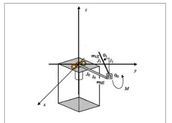
As seen in the literature search, research procedure in the form of algorithms or Pseudocode or other, the effect of time delay can be verified scientifically [2], [4]. The plant that needs to be controlled can be represented as in Figure 1 with various variables as tabulated in appendix A and with the dynamics of the rotary inverted pendulum can be given using Equations 1 and 2. The nonlinear model of the mechanical part of the system has been derived using Newton or the Euler Lagrange formalism. The torque acts as the only control input. Based on the linearized system model, trajectory tracking approach to the problem of changing the angular position of the horizontal arm between an initial and final value while keeping the pendulum around its unstable equilibrium position.

The dynamics of the rotary inverted pendulum are given as [1] and the notations used are same as explained in the work on the same plant.

(3)

0

sin

cos

sin

₀ ₀ ₁2 ₃ ₀

2 1 0 1 1 0

0





M



Cos





M





M

g





M



(1)









2



₂ ₀ ₀ ₀ ₁



0 0 1 1 0 2 3 4 1 0

1

Cos



M

(

M

sin

)



M

sin



2

M

sin

cos



M

(2)

Where in equation 2 refers to the control input which is applied to the shaft of the arm. Mi (i= 0, 1, 2, 3, 4) in equations 1 and 2 are positive system parameters determined as:

1 2 1 1 0 I l m

M   (3)

2 1 1 1 ml L

M  (4)

1 2 1 2 l m

M  (5)

1 1 3 l m

M  (6)

1 2 2 2 2 2 2

4 I l m L m

M    (7)

The plant equations considered under state space representation are as follows:

u A A E bG E qd E CG E bd                                                                         2 1 1 0 1 0 1 0 1 0 0 0 1 0 0 0 0 1 0 0 0 0 / / 0 0 / /                 (8)

Where

a



J

_eq



mr

2

;

b



mLr

;

4

/

3

;

2

ML

C



d



mgL

;

2

;

b

ac

E





The dynamics of the plant are modified to accommodate the time delay influence on the system. So, taking the four states that represent as follows a fifth state is added which will influence the system parameter and the effect of the state is considered as time delay. A

transport delay was incorporated into the system which would be τ1. The time delay parameter would dynamics would involve an additional state defined from the following:

)

2

1

(

)

2

1

(



s





x

₁



s



x

_m (9)

2

)

(

₁ 1









x

m



m



(10)

Where



in equation refers to the time delay in the control input which is applied to the cart position and Xm denotes the modified output state condition. The following assumption is additionally considered along with generic assumptions as in [2] which were never investigated by researchers earlier for a rotary pendulum.

a) A small delay is considered in transmitting the input applied to the pendulum.

(4)

(11)

Where

(12)

(13)

(14)

(15)

(16)

₍₁₇₎

(18)

(19)

3. Predominant Pole Determination Using Flower Pollination

Flower pollination algorithm is a nature-inspired algorithm, based on the pollination of plants. Yang [4] has clearly developed and outlined the advantages based on how pollen gets transferred which becomes the approach for the development of the algorithm. Nature has its vivid variety of plants which have evolved over centuries by a natural pollination process. The method the species of flowers use for evolving is interesting and thought provoking. The movement pattern of pollen from one flowering plant to another is a significant way which could be used for applying it as an algorithm for engineering problems. Biotic, crosspollination may occur at long distance, and the pollinators such as bees, bats, birds and flies can fly a long distance, thus they can considered as the global pollination. In addition, bees and birds may behave as Levy flight behaviour, with jump or fly distance steps obeying a Levy distribution [4]. The algorithm for the pollination is given below where the fitness considered is a cumulative function of all the constraints that are acting on the system.

Algorithm: 1. Initialize population

2. Find the best solution for the designated fitness function (Energy Function)

2 2 2

2 2

)

2

(

)

3

(

*

100

)

1

(

)

2

(

*

100

))

1

(

1

(

E

Z













3. Provide switch probability 4. While N<Generations

a. For all flowers

i) Evaluate levy distribution ii) Evaluate global solution

5. If new solution is better update previous solution 6. Find current best solution

(5)

3. Results and Analysis

The analysis that was done as part of this study is categorized as case studies that varied mainly in terms of Computation time(Tc) and other important parameters such as

a. Time delay

b. Flower pollination parameters (Probability switch for levy distribution, population) The poles are [-2.8 + 2.8i; -2.8 - 2.8i;-30; -40; -60]

Table 1. Flower Pollination Analysis

Case ID

Fitness Value Best Solution Iterations Delay

(Secs)

Tc(Secs)

1 10.28-2.39i -0.87069+0.046i ;0.51183-0.056i ; 0.15285-0.010i 400 4 - 2 -247.89+15928.97i 1.8041-2.13i ; -1.8582+3.4i; -2+0i; 5000 1 8.04 3 -12.9213-15.23i 1.7009-1.06i ;-0.13107+0.38i; -0.2807+0.30i; 10000 1 6.62

4 1.19+0.22i 0.31499+0.00i ; 0.18518+0.01i ; 0.025453+0.01i

400 0.02 42.82

5 -38.80-15.59i 1.0412-0.035i; 1.1717+0.220i ; 1.5025-0.06i 400 1 13.47

Case i) In this the total number of evalutions that were considered was 400 and the best solution that was obtained for the fitness is where the fitness minimum value is indicated in Table I. The poles that were placed using this method are also indicated and table II indicates the two categories in which the levy distribution and population were varied. It was seen that the sensitivity of the responses of the states for variation of population and levy distribution was less. However the significant impact of sensitivity was seen in ST and was high when compared to the sensitivity for flower pollination (Sfp) cases as per category ID #2.

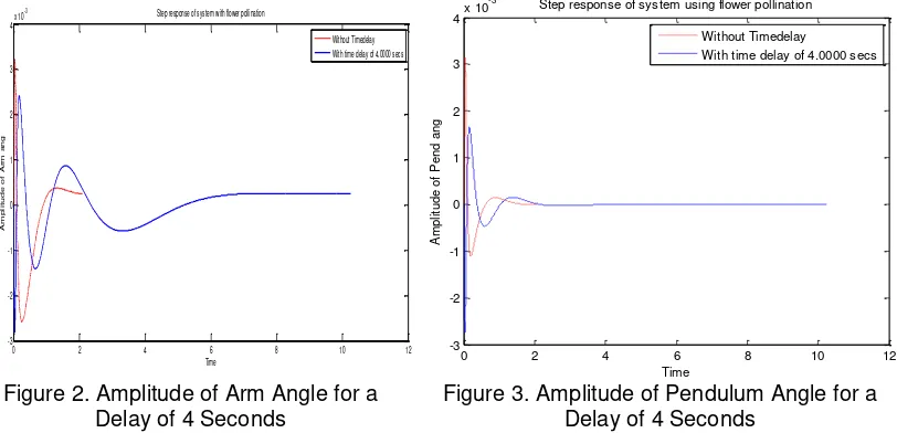
Figure 2. Amplitude of Arm Angle for a Delay of 4 Seconds

Figure 3. Amplitude of Pendulum Angle for a Delay of 4 Seconds

Figure 2 indicates the variation of the arm angle for a delay of 4 seconds and it is clearly seen that the power loss is less and the overshoots with integrated time delay are also relatively less when compared to the case where the power loss is more. The variations is also seen for

0 2 4 6 8 10 12

-3 -2 -1 0 1 2 3 4x 10

-3 _{Step response of system with flower pollination}

Time

A

m

p

li

t

u

d

e

o

f

A

r

m

a

n

g

Without Timedelay With time delay of 4.0000 secs

0 2 4 6 8 10 12

-3 -2 -1 0 1 2 3

4x 10

-3 _{Step response of system using flower pollination}

Time

A

m

p

lit

u

d

e

o

f

P

e

n

d

a

n

g

Table 2. Performance Analysis of Flower Pollination

Category ID Population Levy Distribution Iterations Sensitivity

1 20 .8 20

T

S

=High

2 50 0.4 100

(6)

less overshoot with integrated time delay for the pendulum angle in Figure 3 which indicates that there is less power loss and the energy usage or the control effort in the stabilization of the pendulum about the pendulum is less. The integrated model helps the system to have better control responses with less peak overshoots and relatively faster settling time. This would make the system response smoother with lesser oscillations. This clearly depicts the control efforts are less are the system response is smoother and more robust with the integrated time delay. Incorporating the delay as an independent state has made the overshoots reduce for the states indicating the velocity components for the rotary arm and the pendulum.

The response of the system when the time delay is reduced to 0.002 seconds shows very less variation in the step response of the system using flower pollination. This is imperative in this case as the delay of 0.02 seconds as such on one of the encoders of the system for a such a low value will not effect the system responses in terms of either the control effort required for stabilization, the peak overshoots required or the settling time. This clearly indicate the amount of power loss in this case is almost same to that of the case with no time delay. The responses clearly indicate that the control effort required is very much same and the time delay

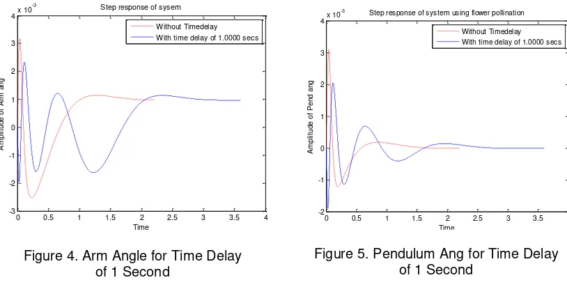
as such doesn’t effect the system response. This indicates that the amount of powerloss involved with the system stabilization is more or less same and the control effort is same in terms of having similar peak overshoots and settling times. Figures 4 and 5 indicate the variations on the rotary arm and pendulum for the system response when a unit delay is considered. As the delay is again increased from a lower value of 0.02 seconds to one unit, the settling times, the peak overshoots become different. This indicates that with the integrated time delay model and by fine tuning the controller gains using settling time conditions we can see that the response has vivid oscillations which indicates in one sense the power losses associated with each of the state. This also indicates that the system dynamic response is affected by the time delay for the settling time and the overshoot, however the integrated model still makes the overshoot reduced because of the inclusion of the additional state into the system matrix.

Figure 4. Arm Angle for Time Delay of 1 Second

Figure 5. Pendulum Ang for Time Delay of 1 Second

Although the variation of the velocities indicated the presence of oscillations which is an indication of more power wastage in the stabilzation of the system, it is achieved at the cost of the overshoots which have been suppressed which becomes a guiding parameter for the system stabilization.

0 0.5 1 1.5 2 2.5 3 3.5 4

-3 -2 -1 0 1 2 3

4x 10

-3 _{Step response of sysem}

Time

A

m

p

lit

u

d

e

o

f

A

rm

a

n

g

0 0.5 1 1.5 2 2.5 3 3.5 4

-2 -1 0 1 2 3 4x 10

-3 _{Step response of system using flower pollination}

Time

A

m

p

lit

u

d

e

o

f

P

e

n

d

a

n

g

(7)

Table 3. Parameters

Parameter Value

Population Size 20

Probability Switch 0.8

Figure 6 Parameter Variation for Different Cases

Table 4. System Response Specifications

Case ID

Peak Overshoot Time(Pend Velocity)

Settling Time (Pend Vel)

Time Delay

Stability Index(0 or 1)

0.06 1.7 4 1

2 0.09 1.7 0.02 1

3 0.09 1.7 1 1

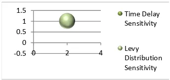
Figure 7. Bubble Chart Analysis

It can be clearly seen from Figures 2 to 5 that the stability achieved in comparison for various time delays was more or less the same but the variation is seen in terms of the control effort required, the power wastage that happens with varied oscillations and less settling time and decreased peak overshoots. Table 4 indicates the settling time and peak overshoot comparisons for the three cases where in case I the time delay was 4 seconds, in case II the time delay was 0.002 seconds and case III the time delay was 1 second. It was observed that the effect of time delay was not predominant. In all the cases it was assume that the probability switch was 0.8 and population was 20. A comparison of various parameters is given in Figure 6. Figure 7 clearly indicates the impact of time delay on sensitivity of the system is high when compared to the parameter variation of pollen levy distribution changes which is not significant based on Table 4 and 3. As seen in Table 4, in all the cases the stability index was high which clearly indicates that the system was stable and was efficiently controlled. Figure 7 is a bubble chart and the relative importance of time delay becomes predominant over the significance of the variation of the flower pollination. Thus, the bubble for the sensitivity as per Table 2 is low and thus the bubble is not noticed for levy distribution sensitivity.

4. Conclusion

From the analysis it can be concluded that flower pollination method is an effective method for the control of stabilization of inverted pendulum wherein the design of the closed loop system poles was achieved by optimization. It can be further applied to complex dynamic systems such as robotic manipulators, space crafts, advanced under actuated ships which require energy efficient methods and this method is directly a method wherein stability index will be high. The sensitivity studies carried out indicate the impact due to the inclusion of time delay into the system parameters significantly affect the system when compared to that of parameter variation of the pollination process. Though pole positions are determined by the flower pollination, the predominance of time delay and design of poles with a given set of flower pollination gives the necessary condition within the limits of time delay and the parameter variation of levy distribution is significantly less. The sensitivity analysis done can be applied to high end complex dynamic robotic systems wherein the sensitivity of cruicial parameters can be

CaseID#1 CaseID#3 0

1 2 3 4

CaseID#1

CaseID#2

CaseID#3

-0.5 0 0.5 1 1.5

0 2 4

Time Delay Sensitivity

(8)

analyzed and thus can be utilized for the understanding and control of these systems. The efficient energy usage depicted through the flower pollination could be applied for a class of robotic systems.

References

[1] K Srikanth, GV Nagesh Kumar. Design and Control of Pendulum with Rotary Arm using Full State Feedback Controller based Particle Swarm Optimization for Stabilization of Rotary Inverted Pendulum Proceedings of 38th National system conference on real time systems –modeling, Analysis and control, JNTU Hyd, Telangana, India. 2014: 59-63.

[2] VP Makkapati, M Reichhartinger, M Horn. The output tracking for dual-inertia system with dead time based on stable system center approach. IEEE Multi-conference on Systems and Control, Conference on Control Applications, Hyderabad, India. 2013.

[3] Xin-She Yang. Flower pollination algorithm for global optimization, Unconventional Computation and Natural Computation, Lecture Notes in Computer Science. 2012; 7445: 240-249.

[4] XS Yang, M Karamanoglu, XS He. Multi-objective flower algorithm for optimization. Procedia in Computer Science. 2013; 18: 861-868.

[5] Qiguo Yan. Output tracking of underactuated rotary inverted pendulum by nonlinear controller," Decision and Control. Proceedings. 42nd IEEE Conference on. 2003; 3: 2395-2400.

[6] Yubai K, Okuhara K, Hirai J. Stabilization of Rotary Inverted Pendulum by Gain-scheduling of Weight and H∞ Loop Shaping Controller. IEEE Industrial Electronics, IECON 2006 - 32nd Annual Conference on. 2006: 288-293.

[7] Jadlovska S, Sarnovsky J. A complex overview of modeling and control of the rotary single inverted pendulum system. Power Engineering & Electrical Engineering. 2013; 11(2): 73-85.

[8] MT Ravichandran, AD Mahindrakar. Robust stabilization of a class of underactuated mechanical systems using time-scaling and Lyapunov redesign. IEEE Transactions on Industrial Electronics. 2011; 58(9): 4299-4313.

[9] Feng Pan, Lu Liu, Dingyu Xue. Double inverted pendulum sliding mode variation structure control based on fractional order exponential approach law. Control and Decision Conference (CCDC). 25th Chinese. 2013: 5077-5080.

[10] Pan Feng, XueDingyu, Chen Dali, Jia Xu. Sliding mode variation structure network controller design based on inverted pendulum. Control and Decision Conference (CCDC), 24th Chinese. 2012; 960-964.

[11] Kumar A, Kumar Y, Mitra R. Reduced dimension fuzzy controller design based on fusion function and application in rotary inverted pendulum. Computing Communication & Networking Technologies (ICCCNT), 2012 Third International Conference on. 2012: 1-5.

[12] Singh Y, Kumar A, Mitra R. Design of ANFIS controller based on fusion function for rotary inverted pendulum. Advances in Power Conversion and Energy Technologies (APCET), 2012 International Conference on. 2012: 1-5.

[13] Kondo T, Kobayashi K, Katayama M. A wireless cooperative motion control system with mutual use of control signals. Industrial Technology (ICIT), 2011 IEEE International Conference on. 2011: 33-38. [14] Barbosa DI, Castillo JS, Combita LF. Rotary inverted pendulum with real time control. Robotics

Symposium, 2011 IEEE IX Latin American and IEEE Colombian Conference on Automatic Control and Industry Applications (LARC). 2011: 1-6.

[15] Alt B, Hartung C, Svaricek F. Robust fuzzy cascade control revised: Application to the rotary inverted pendulum. Control & Automation (MED), 2011 19th Mediterranean Conference on. 2011: 1472-1477. [16] Pan Feng, XueDingyu, Chen Dali, Jia Xu. Sliding mode variation structure network controller design

based on inverted pendulum. Control and Decision Conference (CCDC), 2012 24th Chinese. 2012: 960-964.

[17] Singh Y, Kumar A, Mitra R. Design of ANFIS controller based on fusion function for rotary inverted pendulum. Advances in Power Conversion and Energy Technologies (APCET), 2012 International Conference on. 2012: 1-5.

[18] Kumar A, Kumar Y, Mitra R. Reduced dimension fuzzy controller design based on fusion function and application in rotary inverted pendulum. Computing Communication & Networking Technologies (ICCCNT), Third International Conference on. 2012: 1-5.

[19] Feng Pan, Lu Liu, Dingyu Xue. Double inverted pendulum sliding mode variation structure control based on fractional order exponential approach law. Control and Decision Conference (CCDC), 2013 25th Chinese. 2013: 5077-5080.

[20] Eker J, Astrom KJ. A nonlinear Observer for the Inverted Pendulum. The 8th IEEE Conference on Control Application, Dearborn, USA. 1996

(9)

[22] Heng Liu, Jin Xu, Yeguo sun. Stabilization Controller Design for a class of Inverted Pendulums via Adaptive Fuzzy Sliding Mode Control. Telkomnika Indonesian Journal of Electrical Engineering. 2013; 11(12).