FINITE-DIFFERENCE
APPROXIMATIONS
TO THE HEAT AND DIFFUSION EQUATION
ANDRI HANRYANSYAH
DEPARTMENT OF PHYSICS
FACULTY OF MATHEMATICS AND NATURAL SCIENCES
BOGOR AGRICULTURAL UNIVERSITY
Andri Hanryansyah
NIM G74090039
THE STATEMENT ABOUT
UNDERGRADUATE THESIS
AND INFORMATION RESOURCES AND WITH
COPYRIGHTS GRANTING*
Along with this I declare that this Undergraduate Thesis, which entitled
Finite-Difference Approximations To The Heat And Diffusion Equation are really my works which directed by advisor commission and not yet proposed in any form to any universities or colleges. Information Resources that sourced or quoted from paper or works that is published or unpublished from another writer are already mentioned in the text and imprinted in the bibliography at the end of this Undergraduate Thesis. Along with this I grant my copyrights for my Undergraduate Thesis to Bogor Agricultural University.
ABSTRACT
ANDRI HANRYANSYAH. Finite Difference Approximations to the Heat and Diffusion Equation. Supervised by AGUS KARTONO.
This research review two models of Heat Convection-Diffusion Equation, the Zero-Order model and First-Order model that are derived from advection equation and combined with heat source-sink (S) variable. The Zero-Order model’s S value has linear characteristic as itmakes the system temperature changed linearly. The First Zero model’s S value has exponential characteristic as it makes system temperature changed exponentially. The incompressible flow condition is used in this research. Both models, then solved using two Finite Difference Method,
Forward Time Centered Space (FTCS) and Crank-Nicolson (CN). The convection velocity below 0.3 Mach will not affect the heat transfer process become convection significantly. The incompressible condition makes the convection velocitywould affect the heat transfer process if has a value above 0.3 Mach. The unstability result will be appearing in some simulation condition, especially in FTCS method. It is because the FTCS method is an explicit method which, unconditionally unstable and very sensitive to iteration value, step size, and some additions constant in the equation.
Keywords: advection, convection, Crank-Nicolson, diffusion, Finite Difference
ABSTRAK
ANDRI HANRYANSYAH. Aproksimasi Beda Hingga pada Persamaan Panas dan Difusi. Dibimbing oleh AGUS KARTONO
Penelitian ini mengkaji dua model persamaan difusi konveksi panas, Zero-Order model dan First-Zero-Order model yang diturunkan dari persamaan adveksi dan dikombinasikan dengan variabel sumber atau penyusutan panas (S). Nilai S pada Zero-Order model tidak bergantung suhu , sehingga memiliki karakteristik linear yang menjadikan suhu sistem berubah secara konstan untuk setiap selang waktu. Nilai S pada First-Order model bergantung terhadap suhu, sehingga suhu sistem berubah secara eksponensial untuk setiap selang waktu. Kondisi aliran yang bersifat
incompressible diasumsikan pada penelitian ini. Kedua model tersebut diselesaikan dengan menggunakan dua metoda Beda Hingga. Forward Time Centered Space
(FTCS) and Crank-Nicolson (CN). Kondisi aliran yang incompressible menyebabkan kecepatan konveksi dengan nilai dibawah 0.3 Mach tidak akan mempengaruhi proses transfer panas menjadi konveksi secara signifikan. Kecepatan konveksi akan mempengaruhi proses transfer panas jika memiliki nilai diatas 0.3 Mach. Hasil yang tidak stabil akan muncul dalam beberapa kondisi simulasi, khususnya pada metoda FTCS. Hal ini dikarenakan metoda FTCS merupakan metoda eksplisit yang secara tanpa syarat tidak stabil dan sangat sensitif terhadap nilai iterasi, ukuran step, dan beberapa nilai konstanta tambahan di dalam persamaan.
Bachelor of Sciences Degree At
Department of Physics
FINITE-DIFFERENCE
APPROXIMATIONS
TO THE HEAT AND DIFFUSION EQUATION
ANDRI HANRYANSYAH
DEPARTMENT OF PHYSICS
FACULTY OF MATHEMATICS AND NATURAL SCIENCES
BOGOR AGRICULTURAL UNIVERSITY
BOGOR
2014
Project Title: Finite-Difference Approximations to The Heat And Diffusion Equation
Name : Andri Hanryansyah NIM : G74090039
Approved by
Dr Agus Kartono Supervisor
Known by
Dr Akhiruddin Maddu Chief of Department of Physics
ACKNOWLEDGEMENTS
The author would like to acknowledge His countless thanks to the Most
The author would wish to take his chance to express his thanks and sincere gratitude to the chase:
1. My Beloved Parents, Rachmat Jehan and Cucu Aisyah, who always give me support.
2. My lovely brothers, Indra Nugraha Ramdhani and Alm. Muhammad Fauzan Nurrahman.
3. Dr. Agus Kartono, my supervisor, who has given his best guidance, advice
University, Who has given guidance and inspiring thought.
5. Dr. Husin Alatas, who has been my Academic Advisor from 3rd semester
Bogor, July 2014
Andri Hanryansyah
Gracious and the Most Merciful, ALLAH subhanawata’ala who always gives His all the best of this life and there is no question about it. Shalawat and Salaam to the Prophet Muhammad SAW and his family. This Undergraduate Thesis is submitted to satisfy one of the requirements in accomplishing the Undergraduate Degree at the Department Physics, Faculty of Mathematics and Natural Sciences in Bogor Agricultural University.
and support to write and finish this Undergraduate Thesis.
4. Dr. Akhiruddin Maddu, Chief of Physics Department, Bogor Agricultural
till 7th semester and inspired me to always give my best.
6. Tony Sumaryada Ph.D , my Undergraduate Thesis editor, who has given critique and advice to my handwriting.
7. All lecturers in Physics Department for their invaluable teaching. 8. Mr. Firman, who has given help for the administration affairs.
9. Arbainah, who always given her best support and helped the writer to finish this Undergraduate Thesis.
10.Esha Ardhie, Iman Noor, and Caesar Riyadi, my best friends who always supported me to finish this Undergraduate Thesis.
11.Mr Adi Sunaryo, who has helped the writer to complete this Undergraduate Thesis.
12.All Physics 46, 47, and 48, who have supported the writer.
TABLE OF CONTENTS
TABLE OF CONTENTS ... vi
TABLE OF FIGURE ... vii
TABLE OF APPENDIX ... viii
INTRODUCTION ... 1
Backgrounds Problem ... 1
Formulation of the Problem ... 1
Research Objective ... 1
The Benefits of Research ... 2
The Scope of Research... 2
BACKGROUND THEORY ... 3
Heat Diffusion Equation ... 3
Convection-Diffusion Equation ... 3
Dirichlet Boundary Condition ... 4
Finite Difference Method ... 4
Forward Time Centered Space Scheme ... 5
Crank Nicolson Method ... 6
METHODS ... 9
Time and Place of Research ... 9
Research Tools ... 9
Research Method ... 9
Research Flowchart ... 10
RESULT AND DISCUSSION ... 11
Heat Convection-Diffusion Simulation Using FTCS ... 11
Heat Convection-Diffusion Simulation Using Crank Nicolson ... 13
Heat Source-Sink Value ... 17
CONCLUSION ... 18
BIBLIOGRAPHY ... 19
APPENDIX ... 20
TABLE OF FIGURE
Figure 1: Mesh on a semi infinite strip used for solution in one dimensional
equation problem.3 ... 5
Figure 2: Four nodes that represent the FTCS calculation process ... 6
Figure 3: Six nodes that represent the Crank-Nicolson calculation step process. ... 7
Figure 4 : Research Flowchart ... 10
Figure 5: A shifted function which represent the advection process11 ... 11
Figure 6: A smoother function, which represents the diffusion process11 ... 11
Figure 7 : Temperature Distribution at 0, 2, 4, 6, 8 and 10 seconds using FTCS method with Zero-Order model (v = 10 m/s & nx = 40) ... 12
Figure 8 : Temperature Distribution at 0, 2, 4, 6, 8 and 10 seconds using FTCS method with First-Order model (v = 10 m/s & nx = 40) ... 12
Figure 9 : Temperature Distribution at 0, 2, 4, 6, 8 and 10 seconds using Crank Nicolson method with Zero-Order model (v = 10 m/s & nx = 40). ... 14
Figure 10 : Temperature Distribution at 0, 2, 4, 6, 8 and 10 seconds using Crank Nicolson method with First-Order model (v = 10 m/s & nx = 40). ... 14
Figure 11 : Temperature Distribution at 0, 2, 4, 6, 8 and 10 seconds using Crank Nicolson method with Zero-Order model (v = 10 m/s & nx = 400). ... 15
Figure 12 : Temperature Distribution at 0, 2, 4, 6, 8 and 10 seconds using Crank Nicolson method with First-Order model (v = 10 m/s & nx = 400). ... 15
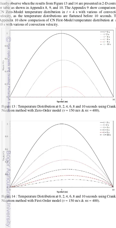
Figure 13 : Temperature Distribution at 0, 2, 4, 6, 8 and 10 seconds using Crank Nicolson method with Zero-Order model (v = 150 m/s & nx = 400). ... 16
Figure 14 : Temperature Distribution at 0, 2, 4, 6, 8 and 10 seconds using Crank Nicolson method with First-Order model (v = 150 m/s & nx = 400). ... 16
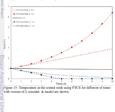
Figure 16: Temperature at the central node using FTCS for different of times with various of k constant, & model are shown. ... 17
TABLE OF APPENDIX
Appendix 1. Example of GUI on Heat Convection-Diffusion MATLAB Simulation Program Main Menu. ... 20
Appendix 2. Example of GUI on Heat Convection-Diffusion MATLAB Simulation Program Input Menu with Simulation Result. ... 20
Appendix 3. Zero-Order and First-Order model formulation from FTCS. ... 21
Appendix 4. Zero-Order and First-Order model formulation from Crank Nicolson. ... 22
Appendix 5. The 3-D Contour plot shows an unstable result of the temperature distribution at various of time using FTCS Zero-Order (left) and First-Zero-Order model (right) with v = 10 m/s, nt = 40, nx = 400, k = 0.2, & α = 0.1 ... 23
Appendix 6. The 3-D Contour plot shows an unstable result of the temperature distribution at various of time using FTCS Zero-Order (left) and First-Zero-Order model (right) with v = 150 m/s, nt
= 40, nx = 40, k = 0.2, & α = 0.1 ... 24
Appendix 7. The 2-D Contour plot shows The Temperature Distribution at t = 0 until 10 seconds using Zero-Order model (left) and First-Order model (right) with Crank Nicolson method (v = 10 m/s & nx = 400) ... 24
Appendix 8. The 2-D Contour plot shows The Temperature Distribution at t = 0 until 10 seconds using Zero-Order model (left) and First-Order model (right) with Crank Nicolson method (v = 150 m/s & nx = 400) ... 24
Appendix 9. Table of Temperature Dsitribution at t = 0 and t = 10 s, using Crank-Nicolson Zero-Order Model with various convection velocity value and k = -0.2 compared to Temperature Distribution using Crank-Nicoloson and Exact method without
Appendix 10. Table of Temperature Dsitribution at t = 0 and t = 10 s, using Crank-Nicolson First-Order Model with various convection velocity value and k = -0.2 compared to Temperature Distribution using Crank-Nicoloson and Exact method without
v and k value. ... 26
1
INTRODUCTION
Backgrounds Problem
The heat-transfer equations play a major role in the modeling of some physical phenomena. These equations are used when attempting to describe heat transport processes and show the heat distribution on it.1 The heat equations are the example of Partial Differential Equations, further the heat equations are belonging to Parabolic Equations that are part of Quasilinear Equations, which is one of the type Partial Differential Equations.2 Some techniques have been developed to find an appropriate simulation method of it as same with natural process.1 Numerical results show that the complete reliability of the proposed algorithms.3
The main concern of this research is to simulate the heat transfer on one dimensional case with the Dirichlet boundary problem. And then, the influence of the convection velocity and heat source-sink value which, is based from mass diffusion equations are given in this simulation and combined with finite-difference methods.1 Some additions from mass advection diffusion equation, hopefully could make a better model for heat transfer.
Formulation of the Problem
1. What is the effect of the convection velocity on heat-transfer process? 2. What is the effect of heat source-sink value on heat-transfer process? 3. What is the effect of the incompressible flow condition on heat-transfer
process?
4. What is the effect of the used by Zero and First-Order Model on heat-transfer simulation result?
Research Objective
1. Investigate and analyze the effect of convection velocity on the heat-transfer process. method and Crank Nicholson method.
2
The Benefits of Research
This research delivers benefits for the field of physics modeling, especially in Heat Transfer modeling. This Research is expected to help researchers and people who desire to learn more about heat transfer phenomena.
The Scope of Research
The Simulation result obtained via two modified heat equation. First, heat equation based on the zero-order diffusion equation. Second, heat equation based on the first-order diffusion equation. Both equations were solved numerically using two Finite Difference Methods, Forward Time Centered Space method and Crank Nicolson method. There are some assumptions on this simulation, such as the
3
BACKGROUND THEORY
Heat Diffusion Equation
The Heat Diffusion Equation belongs to Parabolic Equations that are part of Quasilinear Equations, which are one of types Partial Differential Equations.2 The equations are usually stated as follows:
∂T ∂t = α
∂2T
∂x2 (1)
The � constant known as thermal diffusivity which is a measure of how fast a material can carry heat away from a higher to lower temperature.4
Convection-Diffusion Equation
Convection-diffusion equation plays a pivotal role in the modeling of some physics simulation where heat or energy is transformed inside a physical system due to two processes: convection and diffusion.5 The convection means the movement of molecules or particles within heat. The diffusion describes the spread of particles through random motion from regions of higher to lower concentration. Besides, this equation can be described as advection-diffusion of quantities such as heat, mass, energy, etc.5 Many people widely used this in analyzing the spread of solute in a liquid flowing through a tube, long range transport of pollutants in the atmosphere, flow in porous media and many more. 6,7,8
Many journals, scientific papers, and books stated that the convection-diffusion equation depending on the context, the same equation can be called as the advection-diffusion equation. 9 The general equation for convection–diffusion usually stated : 8, 9,10
∂T
∂t+∇∙ v⃗T =∇∙ α∇T +S (2)
In the one-dimensional case, the convection-diffusion equation become
∂T
4
phenomena). Otherwise, if the heat inside the system is decreased, means that the reaction inside of it is exothermic (cooling phenomena).
The Convection-Diffusion with Zero-Order Source Sink Terms. The formulas are as follows:
The Convection-Diffusion with First-Order Source Sink Terms, with the formula are as follows:
The difference between both formulas are The Heat Source/Sink from Zero-Order model are not depending on the temperature and the other hand the Heat Source/Sink from First - Order model are dependent with the temperature.
Dirichlet Boundary Condition
In engineering applications, a Dirichlet boundary condition may also be referred to as a fixed boundary condition. 12 In this case, we assumed that the equation has some boundary terms are:
∂T
Finite-Difference Methods (FDM) is numerical methods for approximating solutions of differential equations using finite difference equations. The idea of this method is to divide the whole interval t0 ≤ t ≤ tmax into M segments of width Δt =
(tmax – t0)/M and approximate the first & second derivatives in the differential equations for each grid point by the central difference formulas. However, in order for this system of equations to be solved easily, it should be linear, implying that its coefficients may not contain any term of x.12,13 The finite difference method obtains an approximate solution for T (x, t) at a finite set of x and t. The codes developed in this research based on some literature, the discrete x is uniformly spaced in interval of 0 ≤ x ≤ L such as. 3
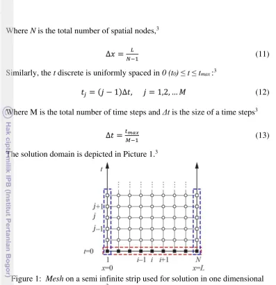
5 Where N is the total number of spatial nodes,3
∆� =
− (11)
Similarly, the t discrete is uniformly spaced in 0 (t0) ≤ t ≤ tmax :3
� = − ∆�, = , , … (12)
Where M is the total number of time steps and Δt is the size of a time steps3
∆� =����
− (13)
The solution domain is depicted in Picture 1.3
As shown in the Figure 1, the black squares with indicated by a red dash border is the location of the known initial value T x,0 = f x . The open squares which indicated by a blue dash border is the location of the known boundary terms
T 0,t =T(L,t). The open circles show the location of the inside points where the finite difference approximation is calculated.3
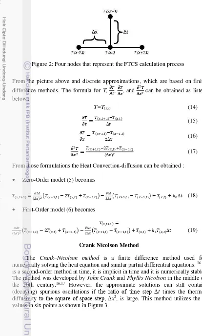
Forward Time Centered Space Scheme
The FTCS (Forward-Time Central-Space) method is a finite difference method used for numerically solving parabolic partial differential equations.14 It is a first-order method in time, explicit in time, and is conditionally stable when applied to the heat equation. When practiced as a method for advection equations, or more generally hyperbolic partial differential equation, it is unstable unless the artificial viscosity is included. The abbreviation FTCS was first used by Patrick Roache.15
FTCS method is usually used in Heat Transfer or Fluid Dynamics Computation. Figure 2 shows four nodes in the grid mesh schematically represent the FTCS calculation process.
6
From those formulations the Heat Convection-diffusion can be obtained : Zero-Order model (5) becomes
��,�+ = �∆�∆� (��+ ,� − ��,� + ��− ,�) −�⃗⃗∆�∆�(��+ ,� − ��− ,�) + ��,� + ∆� (18) First-Order model (6) becomes
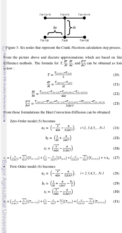
��,�+ = numerically solving the heat equation and similar partial differential equations. 16 It is a second-order method in time, it is implicit in time and it is numerically stable. The method was developed by John Crank and Phyllis Nicolson in the middle of the 20th century.16,17 However, the approximate solutions can still contain (decaying) spurious oscillations if the ratio of time step Δt times the thermal diffusivity to the square of space step, Δx2, is large. This method utilizes the T values in six points as shown in Figure 3.
7
From those formulations the Heat Convection-Diffusion can be obtained: Zero-Order model (5) becomes
= −4∆�⃗⃗⃗⃗⃗⃗ −� ∆�� , i=2, 3,4,5,... N-1 (24)
= ∆�+ ∆�� ( )
= 4∆�⃗⃗⃗⃗⃗⃗ −� ∆�� ( )
= ∆�� +4∆�⃗⃗⃗⃗⃗⃗ (�� �− ,�) + ∆�− ∆�� (��,� ) + ∆�� −4∆�⃗⃗⃗⃗⃗⃗ (�� �+ ,� ) + + ( ) First-Order model (6) becomes
= −4∆�⃗⃗⃗⃗⃗⃗ −� ∆�� , i= 2 3,4,5,.. N-1 (28)
= ∆�+ ∆�� − ( 9)
= 4∆�⃗⃗⃗⃗⃗⃗ −� ∆�� ( )
8
Using Dirichlet Boundary Condition in equation (7) (8) and (9)
= , = , = � ,� =
= , = , = � ,� =
The initial temperature distribution on this research project is considered by T x, 0 = f x = Sin πx L⁄ ( )
9
METHODS
Time and Place of Research
This research was held from March 2013 until January 2014 and takes the places at the Computation Physics Laboratory, Department of Physics, Faculty of Mathematics and Natural Sciences, Bogor Agricultural University.
Research Tools
The main tools in this research are DELL Inspiron N4030 Notebook with specification Intel Core-i3 @2. 53 GHz Processors, 2 GB of RAM, Windows Blue (8.1) Operating System and some software that already installed, such as: Microsoft Office 2010, GIMP, Sublime 2 Text Editor, and MATLAB™ 2012b.
Research Method
Literature Study
Literature study was done in order to understand the mechanism of heat transfer and the effect of convection-diffusion and the numerical methods to solve partial differential equation. Moreover, this literature study would make easier the process of result analysis of the program and correlate it with the heat transfer and the diffusion equation.
Formulating the Equation
Some parameters in heat convection-diffusion such as, convection velocity and Heat Source-Sink, are written into the equation in mathematical form and added into the ordinary heat diffusion equation. After the heat convection-diffusion with some parameter has been written in a new equation. Then, the equation is discretized using the Finite Difference Method. The Dirichlet Boundary Condition (Fixed-Boundary) was used as initial and boundary condition.
Simulation Using MATLABTM Software
10
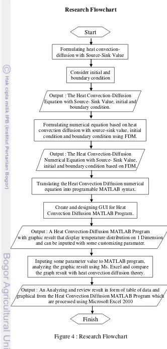
Research Flowchart
Figure 4 : Research Flowchart Start
Formulating heat convection- diffusion with Source-Sink Value
Consider initial and boundary condition
Output : The Heat Convection-Diffusion Equation with Source- Sink Value, initial and
boundary condition.
Formulating numerical equation based on heat convection diffusion with source-sink value, initial
condition and boundary condition using FDM.
Output : The Heat Convection-Diffusion Numerical Equation with Source- Sink Value, initial and boundary condition based on FDM.
Translating the Heat Convection Diffusion numerical equation into programable MATLAB syntax.
Create and designing GUI for Heat Convection Diffusion MATLAB Program.
Output : A Heat Convection-Diffusion MATLAB Program with graphic result that display temperature distribution on 1 Dimension
and can be inputted with some customizing paramater.
Inputing some parameter value to MATLAB program, analyzing the graphic result using Ms. Excel and compare
the graph result with heat convection diffusion theory.
Output : An Analyzing and review result in form of table of data and graphical from the Heat Convection Diffusion MATLAB Program which
are processed using Microsoft Excel 2010
11
RESULT AND DISCUSSION
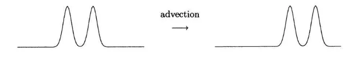
The advection (convection) diffusion equation are underlies the law of mass conservation, it is also called a mass balance equation. Then, it is easily seen that the initial function (initial temperature distribution) at (x,0) is merely shifted in time and velocity v won’t change the function shape as shown in Fig. 5
Fig. 5 shows that the function shifted from the initial function position. 11 The positive value of v used on the Fig. 5, which shows the shift’s direction from left to right and if v use a negative value, the shift’s direction will move from right to left. Consider if the diffusion equations are the only part of the equation with α value is greater than 0, with α denoting the heat conductivity or thermal diffusivity.4,11 The graphic result will mainly interpret the heat convection-diffusion equation as the result of molecular diffusion caused by Brownian motion of particles.11
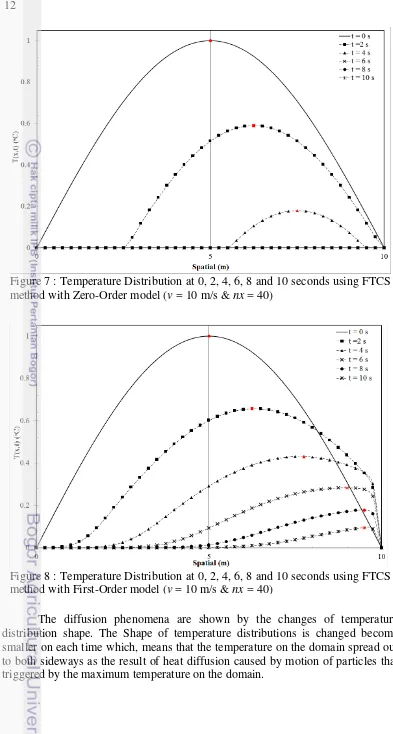
Heat Convection-Diffusion Simulation Using FTCS
Generally the length of mesh L = 10 m is considered. The following parameter input are introduced: thermal diffusivity α = 0.1 (m2/s), mesh iterations
nx = 40, time iterations nt = 40, tmax = 4 s, k constant = -0.2 and convection velocity
v = 10 m/s. The minus sign at k constant means that the system is in the cooling process. The initial temperature distribution in the domain at t = 0 s is of the form (32).
Figure. 7 show the temperature distributions in the domain of x for different of times using FTCS Method with Zero-Order model. Figure. 8 show temperature distributions in the domain of x for different of times using FTCS Methods with First-Order model. The different values of times are shown in both of the figures. Both figures show the convection phenomena which, shown by the temperature distributions are shifting on each time. The maximum temperature on each temperature distribution that indicated by a red sign. The convection phenomena can be seen from the maximum temperatures move in the convection velocity direction.
Figure 5 : A shifted function which represent the advection process11
12
The diffusion phenomena are shown by the changes of temperature distribution shape. The Shape of temperature distributions is changed become smaller on each time which, means that the temperature on the domain spread out to both sideways as the result of heat diffusion caused by motion of particles that triggered by the maximum temperature on the domain.
Figure 7 : Temperature Distribution at 0, 2, 4, 6, 8 and 10 seconds using FTCS method with Zero-Order model (v = 10 m/s & nx = 40)
13 Even though, those all results are not consistent with the theory that considers an incompressible flow. It means in any pressure variations the volumes are constant and in mathematically the v or convection will not affect until the v
value is greater than 0.3 Mach (110 m/s). Both figures result shows that convection velocity= 10 m/s is enough to affect the heat-transfer process become convection process. It is opposite with the theory which stated a low v value which has a value less than 0.3 Mach. So, it won't affect the heat-transfer process become convection process.11 A huge value of iteration should be inputted on simulation, in order to make the simulation result become more accurate. Other parameters such as nt, tmax,
L, α, and v are inputted with the same value at first simulation.
Unfortunately the FTCS can't afford a huge iteration value or very small step size value. It’s because the FTCS is considered as explicit numerical method.4 The unstability calculation result from the FTCS method (both for Zero-Order and First-Order) are shown in Appendix 6. The FTCS method is also could become unstable if some parameter in simulation has been inputted with unusual value, for example, Appendix 7 shows an unstable result graphic of FTCS calculation which, has been inputted with v = 150 m/s.
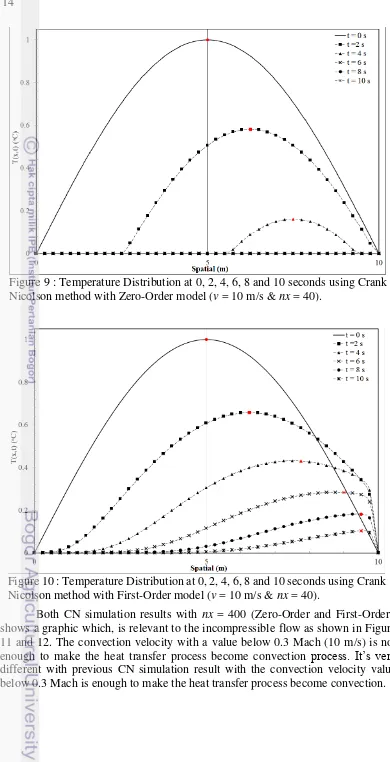
Heat Convection-Diffusion Simulation Using Crank Nicolson
The heat convection-diffusion simulation terms for CN are same as FTCS does. The length of mesh L = 10 m is considered. The following parameter input are introduced: thermal diffusivity α = 0.1 (m2/s), mesh iterations nx = 40, time iterations nt = 40, tmax = 4 s, k constant = -0.2 and convection velocity v = 10 m/s. The minus sign at k constant means that the system is in the cooling process. The initial temperature distribution in the domain at t = 0 s is of the form (32).
Figure. 9 show the temperature distributions in the domain of x for different of times using CN Method with Zero-Order model. Figure. 10 show temperature distributions in the domain of x for different of times using CN Methods with First-Order model. The different values of times are shown in both of the figures. Both figures show the convection phenomena which, shown by the temperature distributions are shifting on each time. The maximum temperature on each temperature distribution that indicated by a red sign. The convection phenomena can be seen from the maximum temperatures move in the convection velocity direction.
14
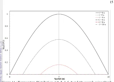
Both CN simulation results with nx = 400 (Zero-Order and First-Order), shows a graphic which, is relevant to the incompressible flow as shown in Figure 11 and 12. The convection velocity with a value below 0.3 Mach (10 m/s) is not enough to make the heat transfer process become convection process. It’s very different with previous CN simulation result with the convection velocity value below 0.3 Mach is enough to make the heat transfer process become convection.
Figure 9 : Temperature Distribution at 0, 2, 4, 6, 8 and 10 seconds using Crank Nicolson method with Zero-Order model (v = 10 m/s & nx = 40).
15
The convection velocity would affect the heat transfer process if the convection velocity value is above 0.3 Mach. Then, in order to prove that. In this simulation, the convection velocity with a value above 0.3 Mach is considered, v = 150 m/s. Both graphic results show a relevant result with the incompressible flow terms. The convection velocity with a value above 0.3 Mach would affect the heat transfer process become convection process. The Convection phenomena will Figure 11 : Temperature Distribution at 0, 2, 4, 6, 8 and 10 seconds using Crank Nicolson method with Zero-Order model (v = 10 m/s & nx = 400).
16
clearly observe when the results from Figure 13 and 14 are presented in 2-D contour or table as shown in Appendix 8, 9, and 10. The Appendix 9 show comparison of CN Zero-Model temperature distribution in t = 4 s with various of convection velocity, as the temperature distributions are flattened before 10 seconds. The Appendix 10 show comparison of CN First-Model temperature distribution at t = 10 s with various of convection velocity.
Figure 13 : Temperature Distribution at 0, 2, 4, 6, 8 and 10 seconds using Crank Nicolson method with Zero-Order model (v = 150 m/s & nx = 400).
17
Heat Source-Sink Value
From the previous section, the result has shown that The Zero-Order’s model (both for FTCS and CN) temperature distributions are faster to being flattened than The First-Order’s model result. The result differences between both models are caused by heat source-sink value that used in both methods.The Zero-Order model uses a Heat Source-Sink value, which causes the temperature of the system changed constantly at each time. The k constant on Zero-Order model are not depends with temperature on the system. The Heat Source-Sink value on the First-Order model is not constant. It depends with the temperature on the system. The Heat Source-Sink value will change if the temperature value is changes.
The simulation has been run with a non - convection term. So, it makes easier to analyze. The midpoint temperature in this simulation is used as a tracking point for heat source sink phenomena. The k constant on First-Order would make a heat sink value that decreased each time step if the systems are in cooling process as shown by the blue curve in Figure 16 and 17. It is because the k constant in the First - Order model used as multiplied factor to produce heat sink value. The heat sink value becomes smaller each time step and become saturated. This cooling curve has a same trends result with the cooling curve based on newton laws of cooling.16 Meanwhile, the k constant would produce a bigger heat source value each time step if the systems are in the heating process as shown on Figure 16 and 17 the temperature increased exponentially.
18
CONCLUSION
A Heat Convection-Diffusion Equation are derived from the heat diffusion equation, advection equation and combined with heat source-sink (S) value. The S
value is a constant which defines a reaction inside the system are exothermic or endothermic. The incompressible flow is used as the condition in this simulation. The Equation categorized into two models. First, the Zero-Order model with the S
value also defined as k constant. Second, the First-Order model with the S value in the equation depends on system temperature (T) value. Both models, then solved using two Finite Difference Method, Forward Time Centered Space (FTCS) and Crank-Nicolson (CN). The Zero-Order model’sS value has linear characteristic as
S of the model makes system temperature changed linearly. The First Zero model’s
S value has exponential characteristic as S on the model makes system temperature changed exponentially. The incompressible flow condition makes the convection velocity with a value below 0.3 Mach will not affect the heat transfer process become convection significantly. The convection velocity would affect the heat transfer process if has a value above 0.3 Mach. The unstability will be appear in some simulation, especially in FTCS method. It is because the FTCS method is an explicit method which, unconditionally unstable and very sensitive to iteration value, step size, and some additions constant in the equation.
19
BIBLIOGRAPHY
[1] Danaila, Ionut; Joly, Pascal; Kaber, Sidi Mahmoud; Postel, Marie;. An Introduction to Scientific Computing. Berlin: Springer, 2007.
[2] Matthews, John H; Fink, Kurtis D.;. Numerical Methods Using MATLAB.
London: Pearson, 2004.
[3] Recktenwald, Gerald W.;. Finite-Difference Approximations to the Heat Equation. Portland-Oregon: Portland State University, 2004.
[4] Lienhard IV, John H.; Lienhard V, John H. A Heat Transfer Textbook Third Edition. Massachussets: Phlogiston Press, 2003.
[5] Mohammadi, Reza. "Exponential B-Spline Solution of Convection-Diffusion Equations." (Applied Mathematics and Computation) 2013. [6] Dehgan, M. "Weighted Finite Difference Techniques for the
One-Dimensional Advection Diffusion Equation." (Applied Mathematics and Computation) 147, no. 2 (2004): 307-319.
[7] R. C., Mittal and R. K., Jain. "Redefined Cubic B-Splines Collocation Method for Solving Convection-Diffusion Equations." (Applied Mathematical Modelling) 2012.
[8] M. K. , Kadalbajoo and P. , Arora. "Taylor-Galerkin B-Spline Finite Element for the One-Dimensional Advection-Diffusion Method for the One-Dimensional Advection-Diffusion Equation." (Numerical Methods for Partial Differential Equations) 26, no. 5 (2010).
[9] Bejan A. Convection Heat Transfer. Wiley, 2013.
[10] Salkuyeh, Davod Khojasteh. "On The Finite Difference Approximation To The Convection-Diffusion Equation." (Elsevier) 2006.
[11] Hundsdorfer , Willem; Verwer, Jan;. Numerical Solution of Time-Dependent Advection-Diffusion- Reaction Equations. Edited by La Jolla R.Bank, La Jolla R.L. Graham, Wurzburg J.Stoer, Kent R.Varga, & Tubingen H.Yserentant. New York: Springer, 2003.
[12] A., Cheng; D. T., Cheng;. "Heritage and Early History of The Boundary Element Method." Engineering Analysis with Boundary Elements (Elsevier), no. 29 (February 2005): 268-302.
[13] Kaw, Autar, and E. Eric Kalu. Numerical Methods with Applications.
Florida: http://www.autarkaw.com, 2008.
[14] Tannehill, John C.; Anderson, Dale A.; Pletcher, Richard H.;.
Computational Fluid Mechanics and Heat Transfer. 3rd. London: Taylor & Francis, 2011.
[15] Roache, Patrick;. Fundamentals of Computational Fluid Dynamics.
London: Hermosa Pub, 1998.
[16] Cebeci, Tuncer. Convective Heat Transfer. 2nd Rev. California: Horizon Publishing, 2002.
20
APPENDIX
Appendix 1. Example of GUI on Heat Convection-Diffusion MATLAB Simulation Program Main Menu.
21
Appendix 3. Zero-Order and First-Order model formulation from FTCS. The formula for T, ��
From those formulations the Heat Convection-Diffusion can be obtained : Zero-Order model (5) becomes
��,�+ −��,�
22
Appendix 4. Zero-Order and First-Order model formulation from Crank Nicolson. The formula for T, ��
��, �� ��, and
� �
�� Of Crank Nicolson are listed below:
� =��,�+ +��,�
From those formulations the Heat Convection-Diffusion can be obtained: Zero-Order model (5) becomes
��,�+ −��,�
Simplifies it and the equation becomes
−4∆�⃗⃗⃗⃗⃗⃗ −� ∆�� (��− ,�+ ) + ∆�+ ∆�� (��,�+ ) + 4∆�⃗⃗⃗⃗⃗⃗ −� ∆�� (��+ ,�+ ) =
First-Order model (6) becomes ��,�+ −��,�
Simplifies it and the equation becomes
−4∆�⃗⃗⃗⃗⃗⃗ −� ∆�� (��− ,�+ ) + ∆�+ ∆�� − (��,�+ ) + 4∆�⃗⃗⃗⃗⃗⃗ −�
The Zero-Order and First-Order model can be represented in matrix format which later will be formulated using tridiagonal matrix.3
23 Where the coefficients of the interior nodes are:
Zero-Order model :
Using Dirichlet Boundary Condition in equation (7) (8) & (9)
= , = , = � ,� =
= , = , = � ,� =
24
Appendix 6. The 3-D Contour plot shows an unstable result of the temperature distribution at various of time using FTCS Zero-Order (left) and First-Order model (right) with v = 150 m/s, nt = 40, nx = 40, k = 0.2, & α = 0.1
Appendix 7. The 2-D Contour plot shows The Temperature Distribution at t = 0 until 10 seconds using Zero-Order model (left) and First-Order model (right) with Crank Nicolson method (v = 10 m/s & nx = 400)
25
Appendix 9. Table of Temperature Dsitribution at t = 0 and t = 10 s, using Crank-Nicolson Zero-Order Model with various convection
26
Appendix 10. Table of Temperature Distribution at t = 0 and t = 10 s, using Crank-Nicolson First-Order Model with various convection
27
Appendix 11. Table of Temperature Distribution at t = 10 s, using CN & FTCS with Zero-Order and First-Order model compared with
28
CURRICULUM VITAE
The writer was born as a first child of Mr. Rachmat Jehan and Mrs. Cucu Aisyah on April 21st, 1991 in Bandung. Astronomy, programming, graphic design, and internet are some of his interests. He has got passed from SMAN 1 Rancaekek in 2009 and accepted as an undergraduate student at Department of Physics, Faculty of Mathematics and Natural Sciences, Bogor Agricultural University from USMI in the same year.