Hydrological Models for Cidanau Watershed

JSPS DGHE

Core University Program in Applied Biosciences

PROCEEDINGS OF THE 3rd SEMINAR

TOWARD HARMONIZATION BETWEEN

DEVELOPMENT AND ENVIRONMENTAL

CONSERVATION IN BIOLOGICAL PRODUCTION

December,

3"'

-

5" ,2004

Serang, Banten (INDONESIA)

Organized Jointly by

Bogor Agricultural University

The University of Tokyo

Government of Banten Province

PI-1

HYDROLOGICAL MODELS FOR CIDANAU WATERSHED

Budi I. Setiawan* and Rudiyanto**

Dept. of Agricultural Engineering, Bogor Agricultural University Kampus IPB Darmaga 16680 Indonesia

Email: *)~udindra@ipb.ac.id, **~lupusae@vahoo.com

Abstract

Hydrological models are necessary in assessing water resources and valuable tool for water resources management. This paper describes applications of Tank model, storage function model and artificial neural networks (ANN) for Cidanau watershed in Indonesia. The Tank model consists of a series of 4 tanks and 5 outflows with 12 independent parameters. Storage function model has 3 parameters. Genetic algorithm (GA) was used for finding the optimum parameters of the tank model and the storage function model. Back-propagation was used in the learning rule of ANN. A series of daily rainfall, evapotranspiration and discharge data for 6

years (1996-2001) from Cidanau watershed was used. The accuracy is evaluated by statistical performance index, the shape of hydrographs and the flood peaks. The results show that tank model, storage function model and ANN are successful in predicting watershed discharge in Cidanau watershed. Comparison of the accuracy of ANN, Tank model and storage function model show that ANN is better than the other models. These hydrological models have been developed in form of application program under Windows and applicable to use in other watershed.

Keywords hydrological models, Cidanau watershed, application program

INTRODUCTION

Hydrological models have become an essential tool for water resources planning, f

development and management. They are for example use to analyze the quantity and quality of stream flow, reservoir system operations, groundwater development and protection, surface water and groundwater conjunctive use management, water distribution system, water use, and a range of water resources management activities (Wurbs 1998). Hydrological models are employed to understand dynamic interaction between climate and land-surface hydrology. An assessment of the impact of climate change on national water resource and agricultural productivity is made possible by the use of hydrological models.

There are several well known general hydrological models in current use in the world. These models vary significantly in the model construct of each individual component process, partly because these models serve somewhat different purposes. HEC- HMS is considered the standard model in the private sector in the United States for the design of drainage system, quantifying the effect of land-use change on flooding, etc. The WATFLOOD model is popular in Canada for hydrologic simulation. TOPMODEL is standard model for hydrologic analysis in many European countries. The Tank models are well accepted in Japan. The Xinanjiang model is commonly used model in China (Singh and Woolhiser, 2002).

models. One of the advantages of such a lumped model is that unlike distributed models it demands only daily rainfall, evapotranspiration and discharge data:

MATERIAL AND METHOD

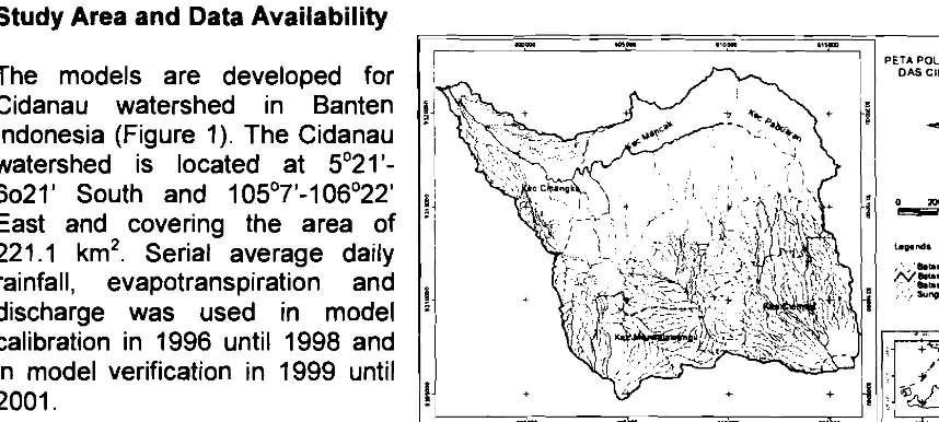
Study Area and Data Availability

DAS CIOANAU

rainfall, evapotranspiration and

[image:3.599.67.496.160.353.2]

calibration in 1996 until 1998 and in model verification in 1999 until 2001.

Figure 1. Cidanau watershed

Tank Model Structure

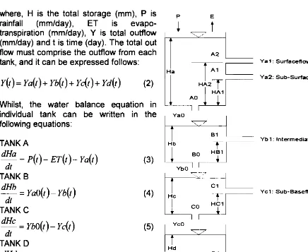
The Tank model comprises of many of simple tanks with outlets arranged vertically one above other. The structure suggested by Sugawara (1974) for the case of humid regions comprises of four tanks in vertical series (Figure 2). This model structure is known as a standard tank model.

Rainfall, the input to hydrologic system, is transformed as output as the stream discharge. The net stream discharge is the sum of the discharge from the outlets of the tank, which are obtained deducting evapotranspiration from rainfall. The intensity rainfall governs the behavior of the model. As such, the water percolating down through the bottom outlets (representing infiltration) and side outlets (runoff in case of first tank, interflow in case of the second tank and base flow in case third and fourth tanks) is derived in a way by parameter of model (Tingsanchali, 2001).

The parameters of tank the Tank model can be classified into three types

1) Runoff coefficient of each tank (A, B, C and D) called as A l , A2, B l , C1 and D l .

2) Infiltration coefficient of each tank called as AO, BO and CO.

3) Storage parameters

-

as height of the side outlets of each tank which include

HA1, HA2, HB1 and HC1.

Parameters of the tank model are as follows and are shown in figure 2 can also divided according to the tank like

TANK A : AO, A l , A2, HA1 and HA2

TANK B : BO, B1 and HB1

TANKC: CO, C1 and HC1 TANKD: D l

The variables as runoff amount from the side outlets (Yal, Ya2, Ybl, Ycl and Ydl, respectively) and infiltration amount from bottom outlets (YaO, YbO and YcO, respectively) are expressed based on the values of parameters mentioned above. The parameters of storage in each tank govern the process as infiltration or runoff depending on the outlet position and the storage depth.

The overall water balance should conform to the following equation:

where, H is the total storage (mm), P is

rainfall (mmlday), ET is evapo-

transpiration (mmlday), Y is total oufflow (mmlday) and t is time (day). The total out flow must comprise the oufflow from each tank, and it can be expressed follows:

Whilst, the water balance equation in individual tank can be written in the following equations:

TANK A

TANK B

TANK C

TANK D

Y a l : Surfaceflw

Ya2: Sub-Surfacellow

B1 I

Y b l : Intermediateflow

f - I--

-YbO I I

1

*

-.:~.::-

-1

Hd

[image:4.599.39.475.164.521.2]

1

Y d l : Baseflow

Figure 2. Schematic Standard Tank model

Storage Function Model

SF model is a simple model for flood runoff. SF model was developed by Kimura (1961) and used successfully since 1961 in all parts of Japan and East Asia. Model input is hydrograph of rainfall and output is hydrograph of discharge.

Runoff is simply expressed by the following storage function:

S = K Q P

(8)

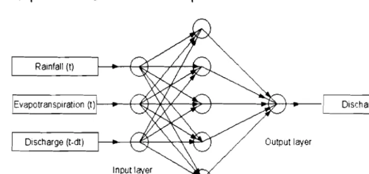
ANN Model Structure

ANN was used for hvdroloaic modelina in the 1990s. Because ANN have abilitv to

I

recursively learn from data and can result in significant savings in time required for model development, they are particularly suited for modeling nonlinear system where

traditional parameter estimation techniques are not convenient.

1

I

Ramfall (t)

Discharge (t-dt) L - \

/

Output layer

-

v

Input

-T

layer

Discharge (1)

w

[image:5.600.92.454.149.320.2]

H~dden layer

Figure 3. Network ANN model

Time delay ANN is used within 3 node in input layer, 5 node in hidden layer and 1 node in output layer. The ANN inputs are rainfall in t time, evapotranspiration in t time and discharge in t-dt time. The ANN output is discharge in t time (Figure 3).

ANN model can be described as follows:

where x is input, v is weight from input node to hidden node, w is weight from hidden node to output node. and f is siamoid function. which is formulated as follows:

where

p

is gain or sigmoid function slope.

I

Model Calibration

Optimization methods have been developed for parameters model estimation. Tank model and SF model use genetic algorithm for finding the optimum of their parameter. Least square criterion was become the objective function. ANN model uses back-propagation for finding their weight. This method was known as power full method, but this method is need long time to get best weight. Serial average daily

1

Model Performance

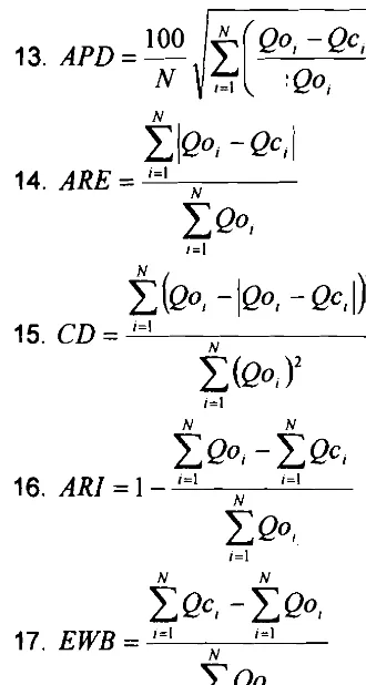
Sixteen common statistics for evaluation of models performance were used R (Coefficient correlation), R~ (Nash-Sutcliffe Coefficient), CD (Coefficient of Determination), RMSE (Root Square Mean Error), MAE (Mean Absolute Error), LOG (Log Root Square Mean Error), Standard x, Squared Standard x, MRE (Mean Relative Error), RR (Root Square Relative Error), NRMSE (Normalized Root Mean Square E m r ) , NME (Normalized Mean Error), El (Model Efficiency), APD (Average Percentage Deviation), ARE (Area Relative Error) and ARI (Annual Run of Index).

l N

4.

M E

_{= -}

x

IQC,

_{- Qo,}

1

_{(1 7 )}

N , = I

2

(log QC, - log QO,

)

4-!-

(QC, - Qo,

)'

10. NRMSE = N , = I

r N

I N I N

2

100

13.

APD

= -

N

14.

ARE

=

'='

,

c

QO, -

c

QC'

16.

ARI

= 1 - '=I !=I

17.

EWB

= '=I

,

r = l

RESULT AND DISCUSSIONS

Tank model, SF model and ANN model prediction and observed hydrograph were

presented in Figure 5, Figure 6 and Figure 7, respectively. The results show that tank

model, storage function model and ANN are successful in predicting watershed

[image:7.598.73.238.74.383.2]

discharge in Cidanau watershed. Highest peak flow analysis show tank model, SF model and ANN can be best reached in 1996, 1997, 2000 and 2001, respectively. Highest peak flow can't be reached by models In 1998 and 1999, respectively. This is happened because the environment in Cidanau watershed is changed.

Table 1 resumes results callbratron and veriflcatlon for ANN model, Tank model and

SF model, with marked values corresponding wlth the best performance according to

the criteria In each row. ANN model become best model for calibration but SF model become best model for verification. Comparison of the accuracy of ANN, Tank model and storage function model show that ANN is better than the other models.

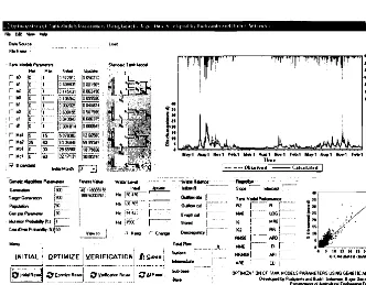
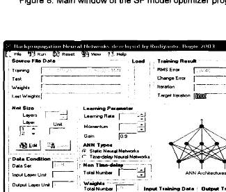
These hydrological models have been developed in form of application program

under Windows, using Borland Delphi 5 programming. Basically this program

receives inputs of date, rainfall, potential evapotransp~ration, and river discharges in mmlday unit. The outputs can be saved in the form of ASCII file for all parameters, error analysls and discharges prediction. The hydrographic and regression curves can be saved in JPG file. Figure 7, 8 and 9 show the main window of the Tank model, the SF model and The ANN model, respectively.

-

- libration

. .

--

. . ... - .

Verification

. .

--

. .

-

-R 0.90 0.88 0.86 0.83 0.81 0.84

R2 0.81 0.77 0.75 0.68 0.65 0.70 ARI 1 .OO 0.99 1 .OO 0.85 1.15 0.86 El 0.88 0.77 0.75 0.61 0.65 0.70

ARE 0.18 0.35 0.37 0.32 0.39 0.30 Table 1. Evaluation of models for hydrograph prediction

Parameter Ca

ANN Tankmoael s t moael ANN l a n ~ m o a e l st moael ;

RMSE 1.17 1.61 1.69 2.21 2.08

APD 0.02 0.03 0.04 0.02 0.03 0.01 MAE 0.58 1.13 1.21 1.19 1.47

Img4

I

1.12 LOG 0.02 0.25 0.36 0.04 0.25 0.1 8 Xi 0.32 0.72 0.77 0.58 0.89 0.54

Xi2 0.26 0.95 1.09 0.62 1.25 0.53 MRE 0.24 0.59 0.62 0.36 0.66 0.31 RR 0.60 1.14 1.21 0.56 0.98 0.43 NRMSE 0.36 0.50 0.52 0.59 0.56 0.52 NME 0.00 -0.01 0.00 -0.15 0.15 -0.14

INITIAL

Fig

T l t M o h l P d m r r .

.... n* r--.. r---.

... - . -... ... -111?1??-.. -. 0 ?!!F ..

ure 7. Main window of the Tank model optimizer program

[image:9.599.91.465.146.583.2] [image:9.599.106.438.333.592.2]

[image:10.599.50.395.70.343.2] [image:10.599.60.385.415.691.2]

Figure 8. Main window of the SF model optimizer program

RMS Err- 1 , :t: 6 ; ;

ChangeErrol --[

Ituatio" ,. " ., .--" ,.---

Tag& rm-...-...-..." .... ^.

N e t S i r s _,.". Laarring Parameter

Layers Rate .... 3

_.-..I

Mom-

I

-G a n (ii3-

a r a 1 : 3 . ]

i:

ANN iype.

i _ . .. . . . . G Static N e u d Nehmkr

i- . . .. . ; r T i n s d d w N w d ..,.,.., Nebwka ... ... ..

1

Data S&

-

1

1 N a n T h - '. '. . .

j Input L q n Unil

7

,

.

ANN Architeclutes

I

,

0'4ULV"u"

-

:=&---

.

14.. T r H g Data O M . . l r . * Z Dala,

CONCLUSSIONS

Hydrological Models that developed is successful in' predicting watershed discharge in Cidanau watershed. Comparison of the accuracy of ANN, Tank model and storage function model show that ANN is better than the other models.

REFRENCES

Fu, L., Neural Networks In Computer Intelligence, McGraw-Hill, Inc, Singapore, 1994.

Heryansyah, A,, M. Y. J. Purwanto and A. Goto, Runoff Modelling in Cidanau Watershed, Banten Province, Indonesia, Proceedings of the 2nd Seminar Toward Harmonization Between Development and Environmental Conservation in Biological Production, JSPS-DGHE Core University

Program in Applied Biosciences, The University of Tokyo, Japan, pp 13-1 8,

2003.

Kimura, T. 1961. The flood runoff analysis method by the storage function model (in

Japanese). The Public Works research Institute, Ministry of Construction. Japan.

Patterson, D. W., Artificial Neural Networks Theory and Application, Printice Hall,

New York, 1996.

Setiawan, B. I., T. Fukuda and Y. Nakano. 2003. Developirlg procedures for

optimization of Tank models parameters. Agricultural Engineering International: the ClGR Journal of Scientific Research and Development.

Manuscript L W 01 006. June 2003.

Sirlg, V. P., and D. A. Woolhiser, Mathematical and Modeling of Watershed

Hydrology. Journal of Hydrologic Engineering. Vol. 7, no. 4. July 21, pp

270-292, 2002.

Sugawara, M., et al. 1974. Tank model and its application to Bird Creek, Wollombi

Brook, Bikin River, Kitsu River, Sanga River and Nam Mune. Research

Note, National Research Center for Disaster Prevention, No. 7 7 , Kyoto,

Japan, 1-64.

Suprayogi, S. 2003. Prediksi ketersediaan air mengunakan tank model dan

pendekatan artificial neural network (studi kasus sub DAS Ciriung Kabupaten Serang). Disertasi Pascasarjana IPB. Bogor.

Tingsanchali, T. 2001. Aplication combined Tank model and AR model in flood

foorecasting . http://www.dhisoftware.com/uc200 1 /papers01 /057/057. htm

Agustus 20031: 13 p.

Wurbs, R. A. 1998. Dissemination of generalized water resources models in the

United States. Water Int., 23, 190-1 98.