DOI: 10.12928/TELKOMNIKA.v13i1.791 211
Nonlinear Filtering with IMM Algorithm for Coastal
Radar Target Tracking System
Rika Sustika1*, Joko Suryana2 1
Research Center for Informatics, Indonesian Institute of Sciences (LIPI) Jl Cisitu 21/154D, Bandung 40135, Indonesia
2
Bandung Institute of Technology (ITB), Jl. Ganesha No 10 Bandung 40135, Indonesia *Corresponding author, e-mail: [email protected]
Abstract
This paper presents a performance evaluation of nonlinear filtering with Interacting Multiple Model (IMM) algorithm for implementation on Indonesian coastal radar target tracking system. On this radar, target motion is modeled using Cartesian coordinate but target position measurements are provided in polar coordinate (range and azimuth). For this implementation, we investigated two types of nonlinear filtering, Converted Measurement Kalman Filter (CMKF) and Unscented Kalman Filter (UKF). IMM algorithm is used to anticipate target motion uncertainty. Many simulations on radar target tracking are developed under assumption that noise characteristic is known. In this paper, the performance of IMM-CMKF and IMM-UKF is evaluated for condition that radar doesn’t know noise characteristic and there is mismatch on noise modeling. Results from simulation show that IMM-CMKF has better performance than IMM-UKF when tracking maneuvering trajectory. Results also show that IMM-CMKF is more robust than IMM-UKF when there is mismatch on noise modeling.
Keywords: CMKF, filtering, IMM, radar, UKF, target tracking
1. Introduction
Primary objective of radar target tracking is to estimate state trajectories of a moving target accurately by using noisy measurement. There are many algorithms for radar target tracking. Kalman filter is the most popular method in modern target tracking systems because of its simplicity and computational efficiency [1].
One of the issues in the design of target tracking system is the choice of the target motion model [2]. On the simplest approximation, the model is assumed as the true dynamic target and a single filter runs based on it. This approach has several obvious flaws because the estimation does not take into account a possible mismatch between the real target dynamic and the filter model [3]. To solve this problem, H.A.P Bloom introduced a safe adaptation or soft switching method that known as Interacting Multiple Model (IMM) [4]. IMM use a bank of filter to estimate state variables of dynamic system. Each filter used different model to characterize a specific motion of a target, which makes it possible to describe a whole motion. By using more than one model, the IMM algorithm is more capable to track targets with motion uncertainty [3].
a very difficult and error-prone process [10]. On 1995, Simon J. Julier and Jeffrey K. Uhlmann proposed another algorithm that known as Unscented Kalman Filter (UKF). In their paper they said that UKF is more accurate and less difficult to implement than EKF as benchmark on nonlinear filtering [7].
In this paper, we present the performance evaluation of IMM method using two nonlinear filtering algorithms based on Kalman filter; those are IMM-CMKF and IMM-UKF, for implementation on coastal radar target tracking system. Evaluation is done to find out the performance of these algorithms in condition when radar doesn’t know the real target dynamic and real noise characteristic. Execution time is also used as evaluation parameter to know the comparison of computational efficiency of the algorithms. Result from this evaluation can be used for implementation on Indonesian coastal radar target tracking system.
2. Model and IMM Algorithm 2.1. Basic Model
The tracking of the single target is based on the choice of a model to describe the dynamic of a target. The simplest target motion model is described in the Cartesian coordinate system by linear discrete-time difference equation with additive noise as [5]
(1)
where A is the state transition matrix (based on model of target dynamic), is state vector on time index k. The state vector ( ) consists of position and velocity or acceleration of the moving target on Cartesian coordinate, i.e, =[ ]T. is process noise that is assumed to be white and zero mean Gaussian with covariance Q.
The target is tracked by ground based radar and provides measurement of range (r) and azimuth (θ). The measurement model is given as [5]
(2)
where is time index, is measurement, and is measurement noise. For this case, when tracking is done on Cartesian coordinate but measurement on polar coordinate, measurement model can be given as [5]
⁄
,
, (3)
where k is time index, is range of the target, is azimuth of the target, and are target position on Cartesian coordinate, and and are measurement noise on polar coordinate, that is assumed to be white and zero mean Gaussian with covariance R.
, (4)
where is range measurement standard deviation and is azimuth measurement standard deviation.
2.2. Interacting Multiple Model
Interacting Multiple Model (IMM) algorithm is a solution for target dynamic uncertainty or to handle a possible mismatch between real target dynamic and filter model. The basic idea of IMM is assume a set of models as possible candidates of the real dynamic target, run a bank of elemental filters, each based on a unique model in the set, and generate the overall estimates by a process based on the results of these elemental filters. On this paper, we used two filters with unique model on each filter; one model used constant velocity (CV) and the other used constant acceleration (CA) model.
Interaction
The mixing probabilities | for each model are calculated as
̅ ∑ (5)
|
̅ (6)
Where is the probability of model Mi and ̅ is nomalization factor. Mixed inputs (means and covariances) of each filter are calculated as
∑ | (7)
∑ | (8)
Filtering
As described before on the introduction, for implementation on coastal radar when tracking on Cartesian coordinate and measurement on polar coordinate, filter that used on this IMM method is nonlinear filtering. Two filtering method has been evaluated, those are CMKF and UKF. These methods will be described latter.
Update Model Probability
In addition to mean and covariance, we compute the likelihood of the measurement for each filter as
Λ v ; , S (9)
and probabilites of each model at time step k are calculated as
∑ Λ ̅ (10)
Λ ̅ (11)
where c is normalizing factor.
Combination
Combination step is to compute state mean and covariance final, and computed with these equations
∑ (12)
∑ (13)
3. Filtering Algorithms
The explanation below is about two filtering algorithms that have been evaluated on this research.
3.1. Converted Measurement Kalman Filter
Time update [8]:
State matrix prediction
| | (14)
Covariance matrix prediction
| | (15)
Measurement update [8]:
Innovation (residual) covariance
| (16)
Kalman gain update
| (17)
State estimation update using last measurement
| | | (18)
Error covariance update
| | (19)
With the converted measurement Kalman filter, polar coordinate measurement first converted to Cartesian coordinate measurement using these equation.
cos (20)
sin (21)
Next, the measurement error matrix, R, needed to be adjusted since data was measured as range and azimuth [9].
(22)
(23)
When
(24)
(25)
(26)
3.2. Unscented Kalman Filter
covariance) of distribution of a variable exactly. After that we propagate the sigma points through the nonlinear function and estimate the moments of transformed variable from them.
For application on coastal radar, when tracking done on Cartesian coordinate while measurement on polar coordinate, time update used equation on Kalman filter time update. Unscented transform is used on measurement update because nonlinearity is on measurement equation.
These equations below are measurement update on Unscented Kalman Filter algorithm [8]. Generation of sigma points
χ | X | (27)
χ | X n λ P| , i , … , n (28)
χ | X n λ P| , i n , … , n (29)
Map sigma points to measurement space
y | h χ | , i=0,...,2n (30)
Predict Z | , covariance S , and cross covariance of state dan measurement P .
Z | ∑ w y | (31)
S ∑ w y | Z | y | Z | R | (32)
P ∑ w χ | X | y| Z | (33)
Filter gain
K P S (34)
Update state dan covariance estimation
X | X | K Z Z | (35)
| | (36)
4. Simulation Scenario
Table 1. Trajectory generation parameters
Time index of maneuvering 1-50 and 71-120 (s)
For initial estimation we used one point approach when the first measurement data used as first estimation of and . First estimation of velocity and on one point approach is assigned as zero [9]. The performance is measured by the percentage fit error (PFE) of position estimation [11]: Every parameter is simulated using 50 runs monte carlo simulation. For evaluation, in this paper we say that performance is good enough for implementation if PFE is under 3%.
Simulations have done with three scenarios, 1st scenario
First scenario is simulation when there is no mismatch on noise modeling. Its mean that noise parameter that is used by filter is the same as real noise that was used on data trajectory and data measurement generation as can be seen on Table 1.
2nd scenario
Second scenario is simulation on condition when there is mismatch on noise modeling. Its mean that noise parameter that is used by filter is different with real noise that is used on measurement trajectory generation. Table 2 shows some parameters for filtering step on 2nd scenario.
Table 2. Filtering Parameters, 2nd Scenario Parameters Value
Probabilities of switching model on IMM .95 . 5 . 5 .95 Prior probability of IMM [0.9 0.1]
3rd scenario
Table 3. Filtering Parameters, 3rd scenario Parameters Value
Psd of process noise (q_cv = q_ca) 0.01 until 1 with interval 0.01 Measurement noise:
Range standard deviation (σr) Azimuth standard deviation (σθ)
10 (m)
0.1 o until 4 o with interval 0.1o
5. Simulation Results
Some figures and tables below are simulation result for two trajectories using three simulation scenarios. Each of simulation has done using monte carlo simulation with 50 runs.
5.1. Non maneuvering trajectory
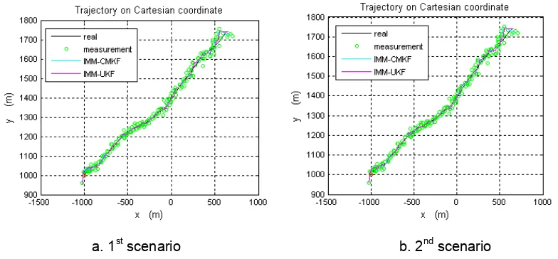
Figure 1 shows performance of CMKF method with IMM algorithm (IMM-CMKF) compare with UKF method with IMM algorithm (IMM-UKF) on nonmaneuvering trajectory. Figure 1.a is trajectory estimation for first scenario when there is no mismatch on noise modeling, and Figure 1.b is trajectory estimation for second scenario, when there is mismatch on noise modeling.
a. 1st scenario b. 2nd scenario
Figure 1. Estimation of non maneuvering trajectory
From Figure 1, the result of simulation using 1st and 2nd scenario nearly the same. A target can be tracked by IMM-CMKF and IMM-UKF with good performance. Estimation of non maneuvering trajectory almost coincides with real trajectory. To see the differences more clearly, we count the PFE as can be seen on Table 4.
Table 4. PFE of nonmaneuvering trajectory estimation
Algorithm PFE (%)
1st scenario 2nd scenario
IMM-CMKF 1.4541 1.7877
IMM-UKF 1.3574 1.7413
From Table 4 we can see that performance of IMM-CMKF and IMM-UKF on 1st scenario is better then performance on 2nd scenario. On all of the scenarios, IMM-CMKF has better performance than IMM-UKF. Results also show that on this type of trajectory, performances of all scenarios are good with PFE fewer than 3%.
this simulation can be seen on Table 3. Simulation result for nonmaneuvering trajectory can be seen on Figure 2. Figure 2.a is simulation result if process noise is varried, and Figure 2.b is simulation if measurement noise is varried.
a. Process noise variation b. Measurement noise variation (σθ)
Figure 2. PFE of position estimation on nonmaneuvering trajectory
As we can see from Figure 2, no significant differences between all two kinds of the filtering algorithms on nonmaneuvering trajectory. Figure 2 shows that on tracking nonmaneuvering target, mismatch on noise modeling is not a big problem because the two algorithms have good performance, with PFE is under 3%.
5.2. Maneuvering trajectory
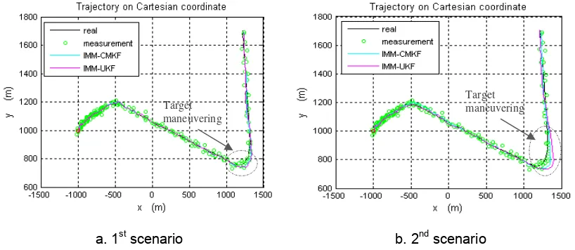
Position estimation using CMKF and UKF with IMM algorithm to track maneuvering target can be seen on Figure 3. Figure 3.a is estimation of maneuvering trajectory on 1st scenario and Figure 3.b is estimation of maneuvering trajectory on 2nd scenario.
a. 1st scenario b. 2nd scenario
Figure 3. Position estimation on maneuvering trajectory
Target maneuvering Target
We can see from Figure 3 that error estimation is large when target is maneuvering. Figure 3.b show that mismatch on noise modelling make errors on trajectory estimation increase, especially when target is maneuvering. IMM-CMKF filtering makes larger error than IMM-UKF on this condition. The result can see clearer by counting the PFE as can be seen on Table 5.
Table 5. PFE of maneuvering trajectory estimation
Algorithm PFE (%)
1st scenario 2nd scenario
IMM-CMKF 1.6475 2.9946
IMM-UKF 1.6312 3.0287
Table 5 shows that PFE of IMM-CMKF and IMM-UKF almost the same for 1st scenario. On 2nd scenario, IMM-CMKF is better than IMM-UKF when target is maneuvering.
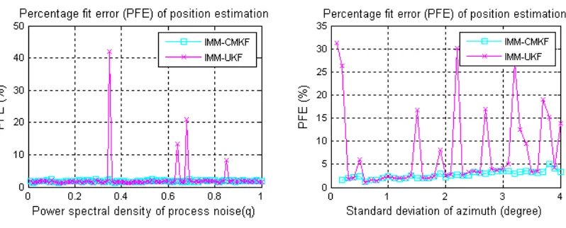
From simulation using 3rd scenario, we have got result as can be seen on Figure 4. Figure 4 shows, when there is a maneuver on target dynamic, mismatch on noise modeling (process noise or measurement noise) make significant influence to trajectory estimation accuracy, especially when filtering using IMM-UKF. From 50 runs monte carlo simulation for each parameter, there are some simulations that the trajectory estimation is divergen. On this situation, radar can’t track the object. This divergence on some simulations makes mean of PFE from 50 runs Monte Carlo simulation using IMM-UKF is more than 3%. On this condition, estimation using IMM-CMKF has better performance. Estimation error (denoted as percentage fit error or PFE) from filtering using IMM-CMKF is lower than estimation error using IMM-UKF. From this simulation we can say that IMM-CMKF is more robust than UKF algorithm for condition when there is mismatch on noise modeling.
a. Process noise variation b. Measurement noise (σθ) variation
Figure 4. PFE of position estimation on maneuvering trajectory
5.3 Execution Time
Table 6. Execution time
Algorithm Execution time (second)
IMM-CMKF 0.077
IMM-UKF 0.285
Table 6 shows that execution time of IMM-CMKF is smaller than IMM-UKF. The execution time for IMM-UKF is about 3.7 times more than IMM-CMKF. This result shows that IMM-CMKF method is simpler than IMM-UKF. IMM-CMKF is simple on this application because the main process is only converting measurement from polar to Cartesian coordinate, and then the system runs Kalman filter based on it. There is no linearization step on this filtering process. On IMM-UKF, there is unscented transformation process that takes more time compare with converting the measurement from polar to Cartesian coordinate.
6. Conclusion
Interacting Multiple Model using Converted Measurement Kalman Filter (MM-CMKF) and Interacting Multiple Model using Unscented Kalman Filter (IMM-UKF) have been considered for implementation on coastal radar, especially for Indonesian coastal radar target tracking system. All two types algorithm, when no mismatch on noise modeling, are able to track the target with good degree of accuracy. IMM-UKF algorithm is a little better than IMM-CMKF algorithm when no mismatch on noise modeling, but with longer execution time. When there is mismatch on noise modeling, IMM-CMKF algorithm has better performance than IMM-UKF algorithm. IMM-UKF still has good performance when no maneuver on target dynamic but the performance is bad when there is maneuver on target dynamic. IMM-CMKF is more robust than IMM-UKF on this condition. Computational complexity of IMM-CMKF is also less than IMM-UKF. From this resulls, it can be concluded that IMM-CMKF is better than IMM-UKF for implementation on coastal radar target tracking system, and IMM-CMKF is suitable to be implemented on Indonesian coastal radar target tracking system.
References
[1] K Rameshbabu, J Swarnadurga, et.al. Target Tracking System Using Kalman Filter. International
Journal of Advanced Engineering Research and Studies. 2012; II: 90-94.
[2] Liu YC, Zuo XG. A Maneuvering Target Tracking Algorithm Based on the Interacting Multiple Models.
TELKOMNIKA Indonesian Journal of Electrical Engineering. 2013; 11(7): 3997-4003.
[3] X Rong L, VP Jilkov. Survey of Maneuvering Target Tracking Part V: Multiple-Model Methods. IEEE
Transactions On Aerospace And Electronic Systems. 2005; 41(4): 1255-1321.
[4] HAP Bloom. An Efficient Filter for Abruptly Changing System. Proceedings of the 23rd IEEE Conference on Decision and Control.1984: 656-658.
[5] Sudesh KK, G Girija, JR Raol. Error Model Converted Measurement and Error Model Modified Extended Kalman Filters for Target Tracking. Defence Science Journal. 2006; 56( 5).
[6] SJ Julier, JK Uhlman. A Consistent, Debiased Method for Converting Between Polar and Cartesian
Coordinate System, The 11th International Symposium On Aerospce/Defense Sensing, Simulation
and Controls. 1997:10-121.
[7] SJ Julier, JK Uhlmann. A New Extension of the Kalman Filter to Nonlinear Systems. The 11th International Symposium On Aerospce/Defense Sensing Simulation and Controls. 1997: 182-193. [8] J Hartikainen, A Solin, AS Sarkka. Optimal Filtering with Kalman Filters and Smoothers: A Manual for
the Matlab Toolbok EKF/UKF. Department of Biomedical Engineering and Computational Science,
Aalto University School of Science, Finland, Version 1.3. 2011.
[9] B Balaji, Z Ding. A Performance Comparison of Nonlinear Filtering Techniques Based on Recorded
Radar Datasets. Proceedings of SPIE. 2009; 7445(1).
[10] Dai H, Dai S, Cong Y, Wu G. Performance Comparison of EKF/UKF/CKF for the Tracking of Ballistic Target. TELKOMNIKA Indonesian Journal of Electrical Engineering. 2012; 10(7): 1692-1699.
[11] VPS Naidu, Girija G, Shanthakumar N. Three Model IMM-EKF for Tracking Targets Executing
Evasive Maneuvers. AIAA Aerospace Meeting and Exhibition. 2007; Paper no. AIAA2007-1204.