ENERGY OPTIMIZATION OF VISION GUIDED MANIPULATOR
FOR OPTIMAL DYNAMIC PERFORMANCE
MUHAMMAD HERMAN JAMALUDDIN
MOHAMED AZMI SAID
MARIZAN SULAIMAN
Paper Presented at The Inaugural International Conference On The Roles Of The Humanities and Sosial Sciences in Engineering 2008, 5-6• December 2008, The Legend Hotel, Malaysia
UNIVERSITI TEKNIKAL MALAYSIA MELAKA
Energy Optimization of Vision Guided Manipulator for Optimal Dynamic
Performance
Muhammad Herman Jamaluddin Kolej Universiti Teknikal Kebangsaan
Malaysia
Mohamed Azmi Said Marizan Sulaiman
Kolej Universiti Teknikal Kebangsaan Malaysia
Kolej Universiti Teknikal Kebangsaan Malaysia
marizanrakutkm. edu. mv
}1erman rtkutl\m.edn mv azn1_isaid "r°z'kutkm.edu.my
Abstract
This paper presents a step on how to optimize the energy and performance of an industrial robot. The project consist of three major phases; (I) theoretical, simulation and practical of jonvard and inverse kinematics/or Fanuc LR lvfate 200iB robot to determine their D-H parameters, (2) optimization of robot movements, and (3) implementation of practical tasks.
The optimization process involves the control of two parameters known as position ofjoint angle (e} and speed of the motor (w}oj the three (3) main axes of the robot. The energy is measured regarding 3 types of categorized movements known as reference, fixed and optimized which do the same repetitive task. Its fonvard and inverse kinematics problems will be simulated using Robotic tools of i\.fatlab 7.0 and Roboguide V2.3.2. The simulation results will be compared with the real practical movements.
Keywords
Manipulators, Optimal Control, Path-Finding, Dynamic Performance.
Introduction
In this project, one of the sensors that are currently being
used in controlling robot mechanism is vision.
Optimal-based control strategies will be developed to perform manipulative actions. This vision guided robot could perform the tasks with improved efficiency using the optimal-based control strategies. The advantages of these optimal control strategies can be seen during performing the tasks wit11 fewer movements of angles, better joint's motor speed and improved time motion that result in more efficient usage of energy.
To find the optimal dynamic perfonnance of a robot, it is important to know the architecture of its kinematics first. From forward or inverse kinematics analysis of that )articular robot, we will obtain an exact position and )rientation for each of its movements. This will help to find he most suitable position and orientation to achieve optimal )erfonnance.
The outline of the paper is as fc.,Jlows. In section 2 a ypical step on searching process of the manipulator's nverse kinematics with given end point is explained in detail. )imulation process is described in section 3 followed by
nergy measurement in section 4 and experimental result in ection 5. Conclusions are stated in section 6.
nverse Kinematics
Inverse Kinematics does the reverse of forward kinematics. Given the end point of the structure, what angles do the
joints need to achieve that end point? It can be difficult, and
there are usually many or infinitely many solutions. Most of the real systems are under constrained, so for a given goal position, there could be infinite solutions (i.e. many different joint configurations could lead to the same endpoint). The
field of robotics has developed many inverse kinematics
systems which, due to their constraints, have closed-fonn solutions.
One of the techniques that had been used to find the exact angle of each joint to reach the goal target is by using the Jacobian method which described briefly in [l].
Inverse Kinematics Analysis of Fanuc
After considering the Jacobian method trough the theoretical calculation based, the analysis which is using the Matlab Robotics tools were done. To find the inverse kinematics in
Matlab, the function that had been used is q
ikine (robot, TJ . This function returns the joint
coordinates for the manipulator described by the object robot
whose end-effectors homogeneous transfonn is given by T. In this project, the robot needs to pick an object at position of [600, 0, -320] and place the object at position of [O, 620, -300].
The complete lists of function regarding this analysis of picking and placing the object using Matlab are as such:
%Entering the D-H parameter information for F.Z\NUC
Ll-link([pi/2 150 0 0 OJ) L2-link i [O セウッ@ o o OJ J L3-link ( [pi/2 75 0 0 OJ) L4-link([pi./2 0 0 290 OJI LS-link ( [4. 7124 0 0 0 OJ I
L6-link([O 0 0 205 OJ)
%Searcr:in:;J for F.Z:\NLIC Position 'a,_nd Orientation Matrix fanuc - robot i{Ll 12 L3 L4 LS L6LJ
%Generate the transform corresponding.to a particular joint
coordinate
q- [ 0 0 0 0 0 0 J
%Forward Kinematic T-fkine (fanuc,q)
Td0transl(-35,0,615)*T
PJ3:ticn
=tra;-isl ;160, , -44D) *Td
セiセy・イウ・@ kゥョセュ。エセ」@
アャ[ゥォゥセ・Hヲ。ョオ」LtャI@
i. F ャウᄋNNZMセ@ ?osi ti on
tセ]tイ。AQウャ@ (-•500, 020,:2'.::·) *Tl
セi@ • (
1.:
16 =
fa nu.:: =
ョ」Nョ。ュセ@ ( axis, RPRREP)
grav [0.00 O.C10 9.81]
ー。イ。Zョ・エセイ@ s
stand;:i_rd
alph3. thst2 E:E'
1. セLイ・LLWYV@ l":•O.OOC10C)O O.OOOO•JC1 0.000000 R Hウエ、セL@ HNQNcゥ{QHjPQセQQI@ ::::sc1.(!(\1:\1=1CiO cャNPPcQHQQjQセェ@ O.C1CJC11)(1(1 F_ (std:
ャNセM[ゥ」L[ウᆱZZᄋ@ ::,_000000 O.C•0(1(11JO 1=1.Q1)<JOOG fセ@ '.std) 1. セᄋWcャWYI@ o. 000000
4. 712400 0. !JOC1C1CJO ,J. OOC1·:10cj Ci. 000000
T
1. !]1=100 Ci
-1. OC1C10
'"
-0. 0000 0Td
l. OOOC; 0
0 -1. 0000
0 -lj. OOOIJ
Ci
Tl
1. 1JOOO 0
0 -1. 0000
0 -0. 0000
0 0
qi
J. 00(1(1(10 290. 00(1(1 R O.OC1(J'.:1CJI) 0.01J1J(I0(1 R Ci. iJOCiOOO ..:::OS. OO(H) R
0 0 0
·) .:J --i:,. 000 l)
rnon .00.2 , -l.C.000 --:! 9: .. 0Q·JO
0 1 .0000
0 TセPNPPPP@
()(1(1(1 o. PPセ@ 3
-1.oocio 120.000CJ ci 1 .0000
D 6(1(\ • PQセQPP@
」セ@ . 0000 0 • OC123 -1. 0000 -3.:·o .0000 0 1 .OOOD
'.stJ) 'std) 'std)
'stdl
(std)
-·) . (J(l(J(J 0. :. 7 3 6 (1. 1848 -0. (l 000 (l. 5583 -0. C1QQ(i
tセ@
1. ゥセjcQHZHQ@ 0
-1 . (1oc1·J 0 NQセQHQQIQセQ@ 6.::>J. (: 1):,:: 3
- ' r l -1. (11·11-'(l 1. 1'j (JIJ(I
The output result above had shown that to go to the target position (pick) at coordinate [600.0,-320] from [440,0.120].
the changes of joint angle as stated in qi are as such:
8::=21.4°
85 = 32°
It is also shown that to go to the target position (place) at
coordinate [0.620.-300] from (600,0.-320]. the changes of
joint angle as stated in q2 are as such:
8:: = 316°
Simulation
The data from the changing angle on the joint will be simulated using Robotic Tools in Matlab. This is to ensure every joint will produce accurate movement and the required end point.
Figure l describes the output of the simulation for the
pick position of simulated Fanuc robot. It shown that the end
point is located at coordinate [600.0,-320]. While Figure 2 shows the output of the simulation for the place position and the end point is located at coordinate [O. 620. -300].
!)
[image:3.608.7.250.87.619.2]J
x
Figure 1 - Simulated movement for picking an object
Figure 2- Simulated movernentfor placing an object
From the data shown. the default position for the pick and place task is in Figure 1 and Figure 2. This default
position is later described fu text as Reference Movement.
There are two types of movement that are modified so that it could achieve the same end point but with different joint
angles. It is later described as Fixed Movement and
Optimized Movement.
Energ:y Measurement
While the robot pick an object at position of (600. 0. -3201
and place it at position of (0, 620. -300]. the ・ョ・イエLセ@ of owrall
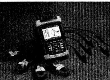
[image:3.608.282.521.251.373.2] [image:3.608.282.524.397.517.2]Quality Analyzer meter as sho\vn in Figure 3. Tltis analyzer meter has 4 BNC-inputs for current clamps and 5 banana-inputs for voltages.
The robot movements for pick and place application involving the use of many motor of its joint and including the energy of its controller that attached together with the robot. So, tltis measurement was done for total of energy usage by the robot and its controller. The energy ' :vas measured at the input cable of the 3-phase power supply. Figure 4 explained
how the connections of Analyzer are made to the 3-phase
[image:4.605.293.503.226.455.2]distribution system and Figure 5 described the real connection of Analyzer to the supply of tlle robot.
Figure 3 - Fluke 434 Three Phase Power Quality Analyzer
-A(L1) MMMMエ。セMMゥゥュセMMMMMᆳB HセI@ MMMMMNGNjゥセセMMKMMNM。エMMMMMMMMᆳ
cHlSIMMZNQセセMMMMKMMヲゥMMBAャャウZZゥャゥNNNMMM
N セセャャゥKMKゥMMMMNKMMKM⦅LMMセMMMᆳ
[image:4.605.43.220.238.366.2]gndセセセNNMNNMセMMKMMKMMセセMMMNZセ@
Figure 4 - Connection of Analyzer to 3-phase distribution system
previously, it is time to test the movement of the manipulator in real application and measure their energy usage . The experiments \Vere divided into three categories of movement which is Reference Movement, Fixed Movement and Optimized Movement. Those were e..\])erimented using real movement of Fanuc robot and run simultaneously together with Roboguide software. Each movement encompasses of
seven steps from P[l] to P[7].
The steps are as such:
•
P[l] - Home position•
P[2] - Pick object•
P[3] - Back to home position•
P[ 4] - Rotate 90° left•
P[5) - PJace object•
P[ 6] - Home position of 90° left•
P[7] - Back to home positionTable 1 - End point coordinates (mm)
Ste1>
x
yz
Pfll
440 0 120P[2] 600 0 -320
Pf3l
440 0 120P[4l
0 440 120Pf 5]
0 620 -300Pf6l
0 440 120Pf71
440 0 120Table l shows the position of end point in coordinate
fonnat of [X,Y,Z] for each step. Those steps were considered
as one cycle of task. Wltile completing the task. the total energy usage by the system were measured and recorded. This measurement depends on process that involves the control of two parameters knovm as position of joint angle
( e) and speed of the motor ( w) of the 3 main axes of the robot. For each categOI}' of moveJUent, the experiments are run
vvith ',
• wl=50% of motor's speed セ カ ゥエィゥョ@ one hour
•
w2=
l 00% of motor's speed within 15 minutes.The experiment of picking and placing the object will be repeated until it reaches the time limit. Within that time frame. the task cycle will be counted and recorded to show the effectiveness of t11ose movements .
Reference Movement
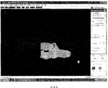
The first category (Reference Movement) was done following the seven steps above . Figure 6 describe the Reference Movement 'vhile picking (P[2]) and placing
(Pf 5]) an object by Roboguide software. This Reference
Movement exactly follows the movement of defa ult inverse kinematics result.
[image:4.605.299.503.348.457.2](a)
[image:5.598.317.493.75.220.2](b)
Figure 6 - References Afovement for (a) picking object, (b) placing object
Fixed Movement
This type of movement '\Vas fixed to minimize the number of motor usage for the joint angle of 3 main axes to reach the target. So, it involves only the movements of motor for Joint
2.
It was done following the seven steps as stated earlier.
Figure 7 describe the reference movement while picking (P[2]) and placing (P[5]) an object. There was a different kind of method on how the robot does the picking task that can be found from Figure 6 (a) and Figure 7 (a). However, the same method is used for the robot placing the object as shown in Figure 6 (b) and Figure 7 (b ). Whatever it is, the robot can still find the same end point target for picking and placing the object.
(a)
[image:5.598.43.217.76.378.2](b)
Figure 5 - Fixed ;'vfovement for (a) picking object, (b} placing object
Optimized Movement
To see the difference from the movement that had been done earlier. this movement were designed to minimize the changing of angle for each joint. Figure 7 shows the Optimized Mm:ement for picking and placing an object.
(a)
(b)
Figure 7 ·· OptimizedMoveme11tfor (a) picking object, (h} placing object
Performance C1;tcria
[image:5.598.318.492.329.645.2] [image:5.598.42.217.608.751.2]-Table ] --Energv measurement for each movement categorv
-
En erg)Motor
Mm ernent Time Speed Cycle Measured
(kWh)
<----Idle l hr
-
-
0147セ@
Reference l hr 50% 135 0.192
Fixed 1 hr 50% 109 0.193
Optimized 1 hr 50% 170 0.190
Idle 15min
-
-
0.037Reference 15min 100% 65 0.057
Fixed 15min 100% 53 0.055
Ootimized 15min 100% 81 0.055
motor's speed.
The data on Table 2 shows the Energy measurement and time motion taken for completing the cycle and repeating it \Vithin specific hour with different speed of the joint's motor.
It is seen that both Optimized Movement of 50% and
100% of motor speed shows the less cycle time taken for completing the task which are 2 l. l 7s and 11. l ls respectively. It also shown that within one hour of repetitive task. it can produce a number of 170 task cycle which more than the other two movements.
The Optimized Movement can nm single task only in 11.lls and a number of 81 cycles within fifteen minutes
\.\ hich produce 32.41 % of energy saving depend on the Reference Movement (50% of motor's speed). That's more efficient than Reference Movement and Fixed Movement. It can be stated here that the Optimized Movement can produce better energy optimization for the entire category.
Conclusion
This paper describes that to find the specific angle of FANUC robotic am1 with given target coordinate, the inverse kinematics solution needs to be applied. The simulation technique and calculation method much helped to achieve the objective of this project. From the experiments that had been executed, it shows that the movement with less task's cycle time and with the fastest of joint motor's speed is more efficient in their overall dynamic perfonnance. The lesser the motor's movement on a joint especially on the three main axes, the lesser the time is taken to complete the task and save energy as well as increase the manipulator's performance. This performance can be really optimized by measuring the smallest energy usage for each of the category of movement.
Energ)- 1 Cycle
1 Cycle Optimization
Usage Energy Usage
Time Percentage
(kWh) (kWh)
-
-
-
-0.045 0.000333 26.67s 0.00%
0.046 0.000422 33.03s -26.61%
0.043 0.000253 21.17s 24.12%
-
-
-
-0.020 0.000312 13.85s 6.54%
0.018 0.000344 16.98s -3.30%
0.018 0.000225 11.1 ls 32.41%
Acknowledgments
The authors wish to acknowledge the financial assistance proYided by Kolej Universiti Teknikal Kebangsaan Malaysia for the overall support of this research.
References
[l} Craig, J.J., 1989. Introduction to Robotics:
Addison-Wesley
[2] Shiller and Sundar, April 1991. Design of Robotic Manipulators for Optimal Dynamic Perfoffilal1ce. In Proceedings of the IEEE International Conference on Robotics and Automation, 344-349. Sacramento, California.
[3J Ngunyen and Graefe, November 2001. Object Manipulation by Leaming Stereo Vision-Based Robots.
In Proceedings of the IEEE International Conference on
Intelligent Robots and Sy stems, 146-151. Maui, Hawaii, USA.
[4] Ngunyen and Graefe, April 2000. Self-Learning Vision-Guided Robots for Searching and Grasping Objects. In Proceedings of the IEEE International Conference on Robotics and Automation, 1633-1638. San Francisco.
[ 5) Bowling and Khatib,-, April 1997. Design of Macro I
Mini Manipulators for 'Optimal Dynamic Perfonnance.
In Proceedings of the IEEE International Conference on
Robotics and Automation, 449-454. Albuquerque, New Mexico.
[6] Herman, Azmi, Marizan and Homg, Jun 2006. Vision Guided Manipulator for Optimal Dynamic Performance. In Proceedings of the IEEE Student Conference on
Research and Development. 147-151. Selangor,
[image:6.625.15.527.94.253.2]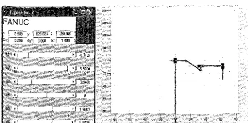
![Table ] -- Energv measurement for each movement categorv](https://thumb-ap.123doks.com/thumbv2/123dok/659482.80749/6.625.15.527.94.253/table-energv-measurement-movement-categorv.webp)
