Dynamic mean-variance portfolio analysis under
model risk
Daniel Kuhn, Panos Parpas, and Ber¸c Rustem
Department of Computing
Imperial College of Science, Technology, and Medicine 180 Queen’s Gate, London SW7 2BZ, UK.
7th October 2007
Abstract. The classical Markowitz approach to portfolio selection is compromised by two major shortcomings. First, there is considerable model risk with respect to
the distribution of asset returns. Especially mean returns are notoriously difficult to
estimate. Moreover, the Markowitz approach is static in that it does not account for the
possibility of portfolio rebalancing within the investment horizon. We propose a robust
dynamic portfolio optimization model to overcome both shortcomings. The model
arises from an infinite-dimensional min-max framework. The objective is to minimize
the worst-case portfolio variance over a family of dynamic investment strategies subject
to a return target constraint. The worst-case variance is evaluated with respect to a set
of conceivable return distributions. We develop a quantitative approach to approximate
this intractable problem by a tractable one and report on numerical experiments.
Key words. portfolio selection, stochastic optimization, robust optimization, bounds, estimation error
1
Introduction
and initial prices of asset n over a given time interval [0, T]. Put differently,
ξn is the factor by which capital invested in asset n grows from time 0 up to timeT. All random objects appearing in this article are defined on a measurable space (Ω,Σ). By convention, random objects (that is, random variables, random vectors, or stochastic processes) appear in boldface, while their realizations are denoted by the same symbols in normal face.
An investor can diversify his or her capital at the beginning of the planning horizon by choosing a portfolio vectorw = (w1, . . . , wN). The component wn of
w denotes the amount of money invested in assetn. In his Nobel Prize-winning work, Markowitz [20] recognized that any such investor faces two conflicting ob-jectives: portfolio ‘risk’ should be minimized while, at the same time, ‘perfor-mance’ should be maximized. Using a benchmark-relative approach, we measure portfolio risk and performance as the variance and expectation of the portfolio excess return (w−wˆ)⊤ξ, respectively. Here, the fixed nonnegative vector ˆw char-acterizes a benchmark portfolio we seek to outperform. As any multi-criterion optimization problem, the Markowitz problem does not have a unique solution. Instead, it has a family of Pareto-optimal solutions, which are found by solving the parametric risk minimization problem
minimize VarQ((w−wˆ)⊤ξ) s.t. EQ((w−wˆ)⊤ξ)≥ρ
(w−wˆ)⊤e= 0
w≥0
(P1)
easy to see that the probability measureQ impacts problemP1 only through the mean value µand the covariance matrix Λ of the asset return vector ξ.
Instead of solving P1, one can determine the efficient frontier also by solving the parametric return maximization problem
maximize (w−wˆ)⊤µ s.t. (w−wˆ)⊤Λ(w−wˆ)≤σ2
(w−wˆ)⊤e= 0
w≥0
(P2)
for different values of the risk target σ2. Sometimes, this alternative model for-mulation is more convenient.
Unfortunately, the Markowitz approach to portfolio selection suffers from two major shortcomings. Firstly, the resulting efficient frontier is not robust with respect to errors in the estimation of µ and Λ. Secondly, the approach is sta-tic and does not account for the possibility of portfolio adjustments in response to changing market conditions. While the lack of robustness leads to an over-estimate, neglecting the dynamic nature of the investment process leads to an underestimate of the achievable portfolio performance. In the present article we will take a closer look at these two inherent deficiencies of the Markowitz ap-proach and discuss possible remedies. Our aim is to propose a framework for the computation of investment strategies that are dynamic as well as robust with respect to uncertain input parameters.
problem where minimization is over a set of dynamic trading strategies and max-imization is over a family of rival return distributions within a given ambiguity set. Min-max problems of this type are extremely difficult to solve. They rep-resent functional optimization problems since investment decisions are functions of the past asset returns. Even worse, the distribution of the asset returns is partially unknown because of estimation errors, and finding the worst-case distri-bution is part of the problem. The approximation of functional min-max prob-lems by finite-dimensional tractable models proceeds in two steps. In Section 4 the constrained min-max problem is reformulated as an unconstrained problem by dualizing the explicit constraints. Section 5 exploits the favorable structural properties of the reformulated model to discretize all rival return distributions simultaneously. We will show that the approximate problem in which the true return distributions are replaced by their discretizations provides an upper bound on the original problem. Moreover, we will establish a transformation that maps any optimal solution of the approximate problem to a near-optimal solution of the original problem. The mathematical tools developed in Sections 4 and 5 will then be used in Section 6 to study a particular investment situation. We will compare Markowitz efficient frontiers obtained under different assumptions about the underlying return distributions and under different rebalancing schemes.
2
Robust portfolio optimization
accurately, it is virtually impossible to measure µ to within workable precision. The reason for this is that return fluctuations over a given time period scale with the square root of period length, which generates a ‘mean blur’ effect [19,§ 8.5]. Hence, the main impediment for the Markowitz approach to produce reasonable results is that the expected returns are flawed with an estimation error, while the efficient frontier is very sensitive to such errors.
To shed light on Michaud’s error maximization property, we assume that the covariance matrix Λ is perfectly known, while the expected return vector is affected by an estimation error. We denote by v2(µ) the optimal value of P2. This representation emphasizes the dependence on the return vectorµ. Next, we assume that µˆ is an unbiased estimator for µ, that is, µˆ is a random variable with EQ(µ) =ˆ µ. By using a simple result about the interchange of expectation and maximization operators, we then conclude that v2(µ) is an upward biasedˆ estimator for v2(µ), the best portfolio return that can be achieved when µ is perfectly known.
EQ(v2(µ)) = EQˆ max
(w−wˆ)⊤µˆ |constraints ofP2
≥ max
(w−wˆ)⊤EQ(µ)ˆ |constraints of P2
= v2(µ)
Thus, using the (unbiased) sample average estimator to approximate µ, for in-stance, leads to a systematic overestimation of the optimal portfolio return and to an upshift of the Markowitz efficient frontier in the risk-return plane.
is referred to asambiguity in the decision theory literature.
The classical Markowitz approach to portfolio selection completely disregards model risk. Put differently, no information about the reliability or the accuracy of the input parameters is passed to the optimization model. To overcome this deficiency, the paradigm of robust portfolio optimization was proposed; a recent survey of the field is provided by Fabozziet al.[8]. The basic idea is to introduce an ambiguity setAwhich contains several probabilistic models orrival probability measures. In order to avoid uninteresting technical complications, we assume that every two measures P1, P2 ∈ A are mutually equivalent, that is, P2 has a density with respect to P1 and vice versa. For the time being, however, we make no additional assumptions about the structure of A. If each P ∈ A is interpreted as a model suggested by an independent expert, then a robust version of the portfolio problem can be formulated as
minimize w∈RN
sup P∈A
VarP((w−wˆ)⊤ξ)
s.t. EP((w−wˆ)⊤ξ)≥ρ ∀P ∈ A (w−wˆ)⊤e= 0
w≥0.
(P3)
This model is robust with respect to all expert opinions. The objective is to min-imize the worst-case variance while satisfying the return target constraint under each rival probability measure. We are not so much interested in the optimal value of problem P3, but rather in its optimal solution. The latter exhibits a
Markowitz model P1 with its well-known shortcomings.
Rustem et al. [24] consider situations in which the ambiguity set is finite. They assume, for instance, that A contains models obtained from different es-timation methods (e.g. by using implied versus historical information). A spe-cialized algorithm is employed to solve the arising discrete min-max problem. El Ghaouiet al. [10] as well as Goldfarb and Iyengar [13] specify the ambiguity set in terms of confidence intervals for certain moments of the return distribution. They reformulate the resulting robust optimization problem as a second-order cone program, which can be solved efficiently. A similar approach is pursued by Ceria and Stubbs [6], who also report on extensive numerical experiments. Pflug and Wozabal [22] determine a ‘most likely’ reference measure ˆP and define A
as some ε-neighborhood of ˆP. Distances of probability measures are computed by using the Wasserstein metric, and the arising continuous min-max problem is addressed by a semi-infinite programming-type algorithm.
3
Dynamic portfolio optimization
So far we have assumed that a portfolio selected at time 0 may not be restructured or ‘rebalanced’ at any time within the planning horizon. In reality, however, an investor will readjust the portfolio allocation whenever significant price changes are observed. In order to capture the dynamic nature of the investment process, we choose a set of ordered time points1 0 =t
1 <· · · < tH =T and assume that portfolio rebalancing is restricted to these discrete dates.
A dynamic extension of the single-period portfolio models studied so far in-volves intertemporal return vectors. By convention, ξh characterizes the asset returns over the rebalancing interval from th−1 to th. Below, we will always as-sume that the ξh are serially independent.2 We define F
h =σ(ξ1, . . . ,ξh) to be 1For notational convenience, we sometimes make reference to an additional time pointt
the σ-algebra induced by the first h return vectors and set F =FH. Moreover, we introduce the shorthand notation ξ = (ξ1, . . . ,ξH) to describe the stochastic return process.
Let us now specify the decision variables needed to formulate a dynamic ver-sion of the portfolio problem. First, we set w−h = (w−1,h, . . . ,w−N,h), where w−n,h denotes the capital invested in asset n at time th before reallocation of funds. Similarly, we definew+h = (w+1,h, . . . ,w+N,h), where w+n,h is the capital invested in asset n at time th after portfolio rebalancing. Notice that these decisions repre-sent random variables since they may depend on past stock price observations. We denote by bn,h and sn,h the amount of money used at time th to buy and sell assets of type n, respectively. As for the asset holdings, we combine these variables to decision vectors bh = (b1,h, . . . ,bN,h) and sh = (s1,h, . . . ,sN,h).
In analogy tow−h and w+h, the random vectors wˆ−h and wˆ+h specify the asset holdings in the benchmark portfolio at time th before and after rebalancing, respectively. However, wˆ−h and wˆ+h are not decision variables. Instead, they constitute prescribed functions of the past asset returnsξ1, . . . ,ξh. Real investors frequently choose an exchange-traded stock index as their benchmark portfolio. Without much loss of generality, we may assume that this stock index is given by theNth asset within our market. In this case, the N −1 first components of the initial portfolio vectorwˆ−1 vanish, while we have
ˆ
w+h =wˆ−h and wˆh+1− =wˆ+h ξN,h+1 for 1≤h < H . (3.1)
Moreover, it is reasonable to normalize the benchmark portfolio in such a way that its initial value corresponds to our investor’s initial endowment, that is,3
(w−1 −wˆ−1)⊤e = 0.
Using the above terminology, we can introduce adynamic version of the robust
3Observe that
w−
portfolio optimization problem P3.
minimize
w−,w+,b,s
sup P∈A
VarP((w+H−1 −wˆ+H−1)⊤ξH)
s.t. EP((w+H−1−wˆ+H−1)⊤ξ
H)≥̺ ∀P ∈ A w+h =w−h +bh−sh 1≤h < H (1 +cb)e⊤bh = (1−cs)e⊤sh ” w−h+1 =ξh+1⊙w+h ” w−h,w+h,bh,sh ≥0, Fh-measurable ”
(P4)
As in the single-period case, the objective is to minimize the worst-case variance of terminal wealth, while satisfying a return target constraint for each rival model
P ∈ A. The second constraint plays the role of an asset-wise balance equation. Notice that proportional transaction costs are incurred whenever the portfolio is rebalanced. We denote bycsand cb the transaction costs per unit of currency for sales and purchases of the assets, respectively. The third constraint thus captures the idea that only a certain percentage of the money received from selling assets can be spent on new purchases. The evolution of money (on a per-asset basis) between the rebalancing dates is described by the fourth constraint. It is the only dynamic constraint coupling successive decision stages. Note that the symbol ‘⊙’ stands for the element-wise multiplication operator. Finally, all decision variables must be nonnegative4 and non-anticipative. The latter requirement means that decisions taken at timeth must beFh-measurable, that is, they may only depend on information about return vectors observed in the past. All constraints are assumed to hold almost surely with respect to some probability measureP ∈ A. The choice of P is irrelevant since the measures in A are pairwise equivalent.
The variance term in the objective function ofP4 is nonlinear in the probabil-ity measureP. This is a potential source of difficulty when designing algorithmic 4The no-short-sales constraints prevent the investor from exploiting potential arbitrage
op-portunities. In an arbitrage-free market, however, these constraints are not necessary to ensure
solution procedures. It turns out, however, that this inconvenient variance term can be approximated by a simple expectation without sacrificing too much accu-racy. In the remainder, we consider a variant of problemP4 in which the variance term is eliminated:
minimize
w−,w+,b,s
sup P∈A
EP([(w−H −wˆ−H)⊤e]2)−ρ2
s.t. constraints of P4.
(P5)
It is easy to verify that the optimal value of P5 constitutes an upper bound on the optimal value of P4. In fact, the performance constraint on terminal wealth translates to the inequality
EP([(w−H −wˆ−H)⊤e]2)−ρ2 ≥ VarP((w−H −wˆ−H)⊤e)
= VarP((w+H−1−wˆ+H−1)⊤ξH).
We will now proceed to investigate problem P5 instead of P4.
port-folio constraints, transaction costs, and other complicating factors are of minor importance.
Cases in which the ambiguity setAcontains more than one model have hardly been addressed in literature. A first approach to tackle such problems is presented in G¨ulpınar and Rustem [11]. In that work, A is assumed to be a finite set of finitely supported models that are representable as scenario trees. The present work goes one step further by allowing A to contain probability measures with an infinite support. These models need to be approximated by scenario trees before the underlying min-max problemP5 can be solved, and the corresponding approximation error has to be estimated carefully.
4
Lagrangian reformulation
Our ultimate goal is to devise a portfolio strategy which is near-optimal and, a fortiori, feasible in P5. The objective value of this strategy will provide a tight upper bound on the minimum of problemP5. In order to facilitate the derivation of a quantitative approximation scheme in Section 5, we now slightly increase the level of abstraction and reformulate P5 as a general stochastic optimization problem under model risk. To this end, we introduce the decision process x = (x1, . . . ,xH) which is defined through5
xh = vec(w−h,w + h,wˆ
− h,wˆ
+
h,bh,sh).
The operator ‘vec’ returns the concatenation of its arguments. Thus, xh has dimension nh = 6N. As the constraints in P5 preclude negative xh, the state space of the process x can be identified with the nonnegative orthant of R6N H.
In standard terminology, such decision processes are also referred to as strategies,
5For technical reasons, it is useful to consider ˆ
w−
h andwˆ
+
h as (degenerate) decision variables.
Note, however, that their values are known a priori for each scenario, since they represent
policies, or decision rules. We define the set of admissible decision processes as
X(F) = \
P∈A
{x∈ ×H
h=1L∞(Ω,Fh, P;Rnh)|x≥0 P-a.s.}. (4.1)
Note that the strategies in X(F) are essentially bounded with respect to all
models P ∈ A and adapted to the filtration F={Fh}H
h=1, that is, they are
non-anticipativewith respect to the underlying return process. Next, we let Ξ denote the state space of the return process, whileX denotes the state space of the (class of admissible) decision processes. Using a suitable cost function c : X → R as
well as a sequence of suitable constraint functionsfh :X×Ξ→Rmh, the dynamic portfolio problemP5is representable as an abstract multistage stochastic program under model risk.
minimize
x∈X(F)
sup P∈A
EP (c(x))
s.t. EP(fh(x,ξ)| Fh)≤0 a.s. ∀P ∈ A, h= 1, . . . , H
(P)
Here, the rules for updating the benchmark portfolio vectors (see e.g. (3.1)) are incorporated as additional constraints. It should be highlighted that the gener-alized problem P accommodates expected value constraints. The corresponding constraint functions are required to be nonpositive in expectation (instead of al-most everywhere), while expectation is conditional on the stagewise information sets. As for problem P5, it is easy to see that the cost and constraint functions can be chosen in such a way that the following regularity conditions hold:
(C1) cis convex and continuous;
(C2) fh is representable as fh(x, ξ) = ˜fh((1, x) ⊗ (1, ξ)), where ˜fh is convex, continuous, and constant in xi⊗ξj for all 1≤j ≤i≤H, 1≤h≤H.
(C3) the processξ is serially independent with respect to all modelsP ∈ A, and its state space Ξ is a compact polyhedron.
The compactness requirement in (C3) can always be enforced by truncating cer-tain extreme scenarios of the return process that have a negligible effect on the solution ofP. Serial independence of returns, on the other hand, is a widely used standard assumption in finance literature. Apart from that, we impose no further restrictions on the return distribution. The conditions (C1)–(C3) are assumed to hold throughout the rest of this paper.
In complete analogy to the setX(F) ofprimaldecision processes , we introduce
a set of dualdecision processes
Y(F) = \
P∈A
{y∈ ×H
h=1L1(Ω,Fh, P;Rmh)|y≥0 P-a.s.}. (4.2)
By construction, a strategy y ∈ Y(F) constitutes a nonnegative F-adapted
sto-chastic process that is P-integrable with respect to all models P ∈ A. Further-more, we denote by Y the state space of the (class of admissible) dual decision processes and define the Lagrangian densityL:X×Y ×Ξ→R associated with
the problem data through
L(x, y, ξ) =c(x) + H X
h=1
yh·fh(x, ξ).
Using the above terminology, we can prove that the stochastic programP under model risk has an equivalent reformulation in terms of the Lagrangian density.
Lemma 4.1. By dualizing the explicit constraints, problem P can be rewritten as the following unconstrained min-max problem:
minimize
x∈X(F) ysup
∈Y(F) sup P∈A
EP(L(x,y,ξ)).
Proof. We generalize an argument due to Wright [26, § 4], which applies when
follows if we can show that the two functionals
Employing standard manipulations, we find
˜
The inequality in the third line reflects the relaxation of the measurability con-straints which requireyhto beFh-measurable for eachh= 1, . . . , H. To prove the converse inequality, we consider a sequence of dual decision strategies {y˜(i)}∞
i=1
5
Approximation
The stochastic optimization problemP under model risk represents a large-scale min-max problem. Minimization is over a set of measurable functionsx∈X(F),
while maximization is over a set of rival models P ∈ A. In the remainder, we will focus on situations in which the ambiguity setA is finite. However, even in this favorable case, problem P remains computationally untractable unless the stochastic return process is discrete (i.e., finitely supported), implying that P
reduces to a finite-dimensional min-max problem. If the return process fails to be discrete, we must approximate it by a suitable discrete process in order to obtain a computationally tractable problem.
The aim of this section is to introduce an approximate return processξu which is supported on a finite subset of Ξ and which relates to the original processξin a quantitative way. In fact, we strive for finding aξu such that the following holds: the optimal value of the min-max problem Pu, which results from the original problemP by substitutingξuforξ, represents a tight upper bound on the optimal value ofP. Our construction ofξu is inspired by Birge and Louveaux [3,§ 11.1] and Kuhn [14, §4]. In the sequel, we use the shorthand notation
ξh = (ξ1, . . . ,ξh) and ξu,h = (ξu1, . . . ,ξuh), h= 1, . . . , H ,
to denote the outcome histories of the processesξandξu, respectively. Moreover, we denote by Ξhthe projection of Ξ on the space spanned by the realizations ofξh, while Ξh stands for the projection of Ξ on the space spanned by the realizations of the return history ξh.
Ω to the state space Ξ. In our setting, we letξ and ξu be coordinate projections.
For every measureP ∈ A, we denote byPξ the marginal distribution of ξ. Since
the sample space is identified with Ξ×Ξ, the joint distribution Pξ,ξu of ξ andξu
coincides withP. In the following, we assume that onlyPξis given a priori, while
the conditional distribution ofξu given ξ, i.e.,Pξu|ξ, is selected at our discretion.
The joint distribution Pξ,ξu is then obtained by using the product measure
the-orem [1, Thethe-orem 2.6.2] to merge Pξ and Pξu|ξ. Although the measures P ∈ A
are partly unknown before we specify the conditional distribution of ξu, there is no problem assuming that they were known already at the outset.
We let the conditional distribution Pξu|ξ be model-independent, that is, we
require it to be equal for all models P ∈ A. The construction of Pξu|ξ relies on
a decomposition into conditional probability distributions Pu
h for 1 ≤ h ≤ H. By definition, Pu
h stands for the distribution of ξ u
h conditional on ξ = ξ and ξu,h−1 = ξu,h−1. By using the product measure theorem [1, Theorem 2.6.2], the building blocksPu
h can later be reassembled to yield Pξu|ξ.
Thus, instead of specifying Pξu|ξ, it is sufficient to prescribe the conditional
probability distributionsPu
h for 1≤h≤H, which will be equal for all P ∈ A. In order to constructPu
h, we select a family of measurable multifunctions [23,§ 14]
Ξh,l: Ξh−1 ⇉Ξh, l = 1, . . . , L ,
such that the following conditions hold for all return histories ξu,h−1 ∈Ξh−1:
(i) simpliciality: the set Ξh,l(ξu,h−1) is either empty or represents a bounded but not necessarily closed simplex for alll;
(ii) disjointness: Ξh,k(ξu,h−1)∩Ξh,l(ξu,h−1) =∅ for all k 6=l;
(iii) exhaustiveness: ∪L
Suitable multifunctions with the postulated properties exist since Ξh is a coordi-nate projection of Ξ, thus representing a compact polyhedron; see (C3). In the sequel, we let{ξh,l,n(ξu,h−1)}N
n=0 be a set ofN+ 1 vectors in Ξh which correspond to the vertices of the simplex Ξh,l(ξu,h−1) if this set is nonempty, or to some ar-bitrary constant vectors, otherwise. Each ξh,l,n can be interpreted as a function from Ξh−1 to Ξh. Since Ξh,l is a measurable multifunction, the vector-valued functions ξh,l,n can be chosen measurably. Next, for any return vector ξh ∈ Ξh we introduce a set of N+ 1 real numbers {λh,l,n(ξh|ξu,h−1)}Nn=0 which satisfy
Eachλh,l,n can be interpreted as a real-valued function on Ξh×Ξh−1. Since the vector-valued functionsξh,l,nare measurable, theλh,l,ncan be chosen measurably, as well. We are now prepared to specify the conditional distributionPu
h. Forξ ∈Ξ
where 1ˆΞ denotes the characteristic function of a set ˆΞ, while δξˆ denotes the Dirac measure concentrated at a point ˆξ. The distribution Pξ,ξu obtained by
combining the marginal distribution of ξ and the conditional distributions Pu h
in the appropriate way has several intriguing properties. Some of these will be explored in Lemmas 5.1 through 5.3.
From now on we denote by Fu the filtration generated by ξu
, that is, Fu = we introduce spaces of approximate primal and dual strategiesX(Fu) andY(Fu), respectively. These are defined in the obvious way by replacing the original filtration F by the approximate filtrationFu in (4.1) and (4.2).
expectations and for all P ∈ A, respectively.
EP(x|F)∈X(F) for all x∈X(Fu) (5.2a)
EP(y|Fu
)∈Y(Fu) for all y∈Y(F) (5.2b)
EP(ξu|F) =ξ (5.2c)
Proof. Let us fix a probability measure P ∈ A. The inclusion (5.2a) is related to the fact that the random vectors {ξui}i≤h and {ξi}i>h are conditionally inde-pendent given{ξi}i≤h for all stage indicesh. Conditional independence, in turn, follows from the serial independence of ξ and the recursive construction of ξu. A rigorous proof of the preceding qualitative arguments is provided in [14,§ 4]. The inclusion (5.2b), on the other hand, is related to the fact that {ξi}i≤h and
{ξui}i>h are conditionally independent given {ξui}i≤h for all h, see [14, § 4]. Next, the relation (5.2c) follows immediately from the definition ofPu
h.
The law of iterated conditional expectations then allows us to conclude that
EP(ξuh|ξ) = EP(EP(ξ u
h|ξ,ξu,h−1)|ξ) = ξh P-a.s. ∀1≤h≤H .
Thus, assertion (5.2c) is established.
The relations 5.2 are crucial for our main result on the approximation of the min-max problemP; see Theorem 5.4 below. It should be emphasized that there is considerable flexibility in the construction of the joint distribution of ξ and
Replacing the original return process byξuand the original filtration byFu in
the min-max problem P yields an approximate min-max problem, which will be denoted byPu. Observe that changing the filtration affects not only the feasible setX(F) but also the information sets in the expected value constraints. Notice
further that Lemma 4.1 remains valid for problemPu with the approximate data process and filtrations. In the remainder of this section we will prove that the optimal valuePu constitutes an upper bound on the optimal value of the original problem P. We first establish two technical lemmas, both of which were proved in [16]. The proofs are repeated, here, in order to keep this paper self-contained.
Lemma 5.2. The following relation holds for suitable versions of the conditional expectations and for all 1≤i < j ≤H, P ∈ A.
EP(xi⊗ξuj|F) = EP(xi|F)⊗ξj for all x∈X(F u
)
Proof. Select a probability measure P ∈ A. Next, fix two stage indices i and
j such that 1 ≤ i < j ≤ H, and let x be an element of X(Fu). By applying
elementary manipulations, we find thatP-almost surely
EP(xi⊗ξuP,j|ξ) = EP(EP(xi⊗ξuj|ξ,ξu,j−1)|ξ)
= EP(xi⊗EP(ξuj|ξ,ξ u,j−1
)|ξ)
= EP(xi⊗ξj|ξ)
= EP(xi|ξ)⊗ξj,
where the third equality follows from the proof of Lemma 5.1.
Lemma 5.3. The following relation holds for suitable versions of the conditional expectations and for all 1≤h≤H, P ∈ A.
EP(fh(x,ξu)|F)≥fh(EP(x|F),ξ) for all x∈X(Fu)
Then, condition (C2) and the conditional Jensen inequality imply that
EP(fh(x,ξu)|F) = EP( ˜fh((1,x)⊗(1,ξu))|F)
≥ f˜h(EP((1,x)⊗(1,ξu)|F))
= f˜h(EP((1,x)|F)⊗(1,ξ))
= fh(EP(x|F),ξ)
almost surely with respect to P. The equality in the third line follows from Lemma 5.2 and independence of ˜fh in all of its argumentsxi⊗ξj with i≥j.
The technical Lemmas 5.1 and 5.3 constitute important ingredients for the proof of the following main result.
Theorem 5.4. Assume problem Pu to be solvable with finite minimum. If xu
solvesPu, thenxˆ = EP(xu|F)is independent ofP ∈ A, feasible inP and satisfies
infP ≤ sup P∈A
EP(c(xˆ))≤infPu.
Proof. Our argumentation relies on ideas from the proofs of Theorem 1 in [14] and Theorem 5.1 in [15]. We use the fact thatxuis an element ofX(Fu), implying via (5.2a) that the conditional expectation EP(xu|F) represents the same element of
X(F) for all P ∈ A.
Another application of the conditional Jensen inequality yields
Here, the second inequality holds by the assumption (5.2b), entailing a relaxation of the dual feasible set. The last line of the above expression corresponds to infPu, which is finite by assumption. This implies that the supremum overY(F) in the first line of (5.3) is also finite, and y = 0 is an optimal solution. Thus,
ˆ
x= EP(xu|F) is feasible in P, and the corresponding worst-case objective value supP∈AEP(c(xˆ)) satisfies the postulated inequalities.
Note that the marginal distribution of the approximate return process ξu is discrete. Since the distribution of ξu conditional on ξ is the same under all rival models P ∈ A, the support of ξu represents a finite set independent of P. Only the probabilities associated with specific discretization points may be model-dependent. Consequently, the approximate problem Pu constitutes a finite-dimensional min-max problem, which is principally amenable to numerical solution. By Theorem 5.4, the optimal value of the approximate problem provides an a priori upper bound on the minimal (worst-case) expected cost. However, an optimal strategy of Pu only prescribes the decisions corresponding to return scenarios in the support of ξu. Such a strategy may fail to be implementable if a generic return scenario from the support of ξ materializes. Put differently, it is a priori unclear how an optimal strategy for the approximate problem can be transformed to a near-optimal strategy for the original problem. Theorem 5.4 provides a particularly satisfactory answer to this question by proposing a policy
ˆ
and whose worst-case expected cost is bracketed by infP and infPu. Note that EP(c(x)) represents an a posteriori estimate of the expected cost associated withˆ
an optimal strategy of problemP under the model P ∈ A. This cost can conve-niently be calculated by Monte Carlo simulation. Since xu is finitely supported, evaluation of xˆ for an arbitrary realization of ξ reduces to the evaluation of a finite sum and poses no computational challenges.
6
Computational results
The mathematical tools developed in Section 5 will now be used to approximately solve robust dynamic portfolio problems of the type P4. Our computational re-sults are based on a market model with N = 5 assets. The asset prices are assumed to follow a multivariate geometric Brownian motion. Thus, the log-returns over equally spaced time intervals are serially independent and normally distributed with given ‘true’ means, standard deviations, and correlations. The monthly means amount to 0.41%, 0.82%, 1.19%, 1.60%, and 1.99%, while the monthly standard deviations are given by 8.5%, 8.0%, 9.5%, 9.0%, and 10.0%. Moreover, the correlations are set to 30% for all pairs of assets.6 The distribu-tional parameters of the log-returns are easily adjusted to other period lengths. In fact, means and variances scale linearly with period length, while covariances remain constant. Thus, our parameters uniquely specify the true modelQ, that is, the true joint probability distribution of the asset returns over the basic re-balancing periods. As discussed in Section 2, however, investors are not aware of the true model. The standard deviations and correlations can be estimated with reasonable accuracy, and therefore it is acceptable to suppose that these parameters are known. Estimation of the means, however, is complicated by the mean blur effect. Hence, only imperfect estimates of the means are available. One can simulate the situation faced by a real investor who estimates the means
based on two years of monthly data: use the true modelQto sample 24 monthly log-returns for all five assets and then determine ‘estimated’ means by calculating the sample average. Experiments of this type were proposed by Broadie [5]. One particular simulation run yields−1.09%, 0.02%, 3.99%, 2.00%, and 2.59% as esti-mated means. These generic values will be used in all our numerical calculations. However, we bear in mind that a different simulation run would have resulted in different values. The estimated means (together with the true standard devia-tions and correladevia-tions) give rise to an estimated model ˆQ, which is known to the investor.
In order to ensure consistency with Broadie’s setup [5], we consider an invest-ment horizon of one month and set the asset holdings in the benchmark portfolio to zero. This implies that the portfolio’s performance and risk are measured in absolute terms. We also assume that rebalancing is allowed atH−1 equidistant time points within the investment horizon. Unless otherwise specified, we set
H = 4 in our numerical calculations. If the investor knew the true modelQ, then he or she would solve the parametric problem7 P
4 with a degenerate ambiguity setA ={Q}. Using Broadie’s terminology, the resulting family of Pareto-efficient portfolios is referred to as the ‘true’ mean-variance frontier. Conversely, if the investor had full confidence in the estimated model ˆQ, then he or she would solve problem P4 using the naive ambiguity set A ={Qˆ}. In that case, the resulting Pareto-optimal curve is termed the ‘estimated’ frontier.
By Michaud’s error maximization property, the estimated frontier lies typ-ically above the true frontier, as is the case in our example (see Fig. 1). By construction, however, no portfolio on the true frontier can possibly be
domi-7Rigorously speaking, the investor will not solveP 4butP
u
5, the discretized tractable version
of problemP5, which provides a conservative upper bound on the original problemP4. If x
u
solvesPu
5, then the investor will implement the strategyxˆ= EP(xu|F), which is independent of P ∈ A and feasible in both P5 and P4. The mean and variance of the terminal wealth
0.01 0.015 0.02 0.025 0.03 0.035 0.04 0.045
0.04 0.045 0.05 0.055 0.06 0.065 0.07 0.075 0.08 0.085 0.09 0.095
Return
Variance
True Frontier Estimated Frontier Actual Frontier Estimated Robust Frontier Actual Robust Frontier
Figure 1: Mean-variance frontiers for different ambiguity sets
nated by any other portfolio with respect to the true modelQ. Hence, evaluating the investment strategy corresponding to any portfolio on the estimated frontier generates a random terminal wealth whose mean and variance (under Q) de-scribe a point below the true frontier. The collection of all mean-variance points obtained in this manner give rise to the ‘actual’ frontier. By construction, the actual frontier necessarily lies beneath the true frontier, see Fig. 1.
Only the estimated frontier is observable in reality. The true and actual frontiers are not observable since their construction is based on the unknown model Q. Loosely speaking, the estimated frontier describes what the investor believes to happen, whereas the actual frontier describes what really happens. As becomes apparent from Fig. 1, these two views of the future may be not at all compatible.
am-biguity sets. In our numerical experiments, A contains the estimated model ˆQ
and several models obtained from shifting the estimated means by ±1.5 stan-dard deviations. This is reasonable since the variance of the estimated means is proportional to the variance of the asset returns. Although the asset returns are positively correlated, it is unlikely that all means are simultaneously over- or underestimated. Thus, we consider only models in which at most three out of the five means are shifted in the same direction.
Solving the parametric problem P4 with this heuristic ambiguity set yields a family of robust portfolio strategies — one for each return target. Any such investment strategy results in a random terminal wealth, whose distribution can be evaluated under each model P ∈ A. The means and variances under the estimated and true models ˆQ and Q give rise to an ‘estimated robust’ and an ‘actual robust’ frontier, respectively. The idea to consider robust frontiers of this type is due to Ceria and Stubbs [6], who obtain similar results to ours in a static one-period case. Loosely speaking, the estimated robust frontier describes what the investor believes to happen, whereas the actual robust frontier describes what really happens. The estimated and actual robust frontiers are much better aligned than their non-robust counterparts. Moreover, they are in a close vicinity of the true Markowitz frontier, see Fig. 1. Thus, using a robust approach is beneficial in two respects: the investor is more realistic about the achievable outcomes than a naive Markowitz investor, and the robust portfolio typically performs better in reality (that is, underQ) than a non-robust Markowitz portfolio.
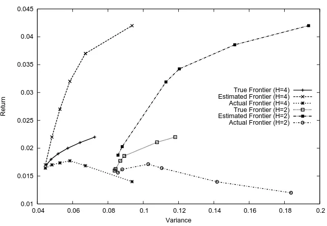
0.01 0.015 0.02 0.025 0.03 0.035 0.04 0.045
0.04 0.06 0.08 0.1 0.12 0.14 0.16 0.18 0.2
Return
Variance
True Frontier (H=4) Estimated Frontier (H=4) Actual Frontier (H=4) True Frontier (H=2) Estimated Frontier (H=2) Actual Frontier (H=2)
Figure 2: Mean-variance frontiers under different rebalancing schemes
when addressing mean-variance portfolio problems.
In this paper, we elaborate a robust and dynamic approach to portfolio opti-mization based on scenario trees. We consider rival probability measures describ-ing the future asset returns and propose a min-max model that predicts realistic portfolio performance and avoids disappointing results. We develop a computa-tional framework for solving this problem approximately and propose methods to control the approximation errors. Our initial numerical experiments show that there are tangible benefits of integrating robust and dynamic approaches in portfolio optimization.
References
[1] Ash, R. Real Analysis and Probability. Probability and Mathematical Sta-tistics. Academic Press, Berlin, 1972.
[2] Bielecki, T. R., Jin, H., Pliska, S. R., and Zhou, X. Y. Continuous-time mean-variance portfolio selection with bankruptcy prohibition. Math. Finance 15, 2 (2005), 213–244.
[3] Birge, J., and Louveaux, F. Introduction to Stochastic Programming. Springer-Verlag, New York, 1997.
[4] Black, F., and Litterman, R. Asset allocation: combining investors’ views with market equilibrium. Technical report. Fixed Income Research, Goldman, Sachs & Co, New York, September 1990.
[5] Broadie, M. Computing efficient frontiers using estimated parameters.
Ann. Oper. Res. 45, 1-4 (1993), 21–58.
[6] Ceria, S., and Stubbs, R. Incorporating estimation errors into portfolio selection: robust portfolio construction. Journal of Asset Management 7, 2 (2006), 109–127.
[7] Chopra, V., and Ziemba, W.The effect of errors in mean, variances, and covariances on optimal portfolio choice. Journal of Portfolio Management
(Winter 1993), 6–11.
[8] Fabozzi, F., Kolm, P., Pachamanova, D., and Focardi, S. Robust portfolio optimization and management. Hoboken: John Wiley & Sons, 2007.
[10] Ghaoui, L. E., Oks, M., and Oustry, F. Worst-case value-at-risk and robust portfolio optimization: A conic programming approach. Oper. Res. 51, 4 (2003), 543–556.
[11] G¨ulpinar, N., and Rustem, B. Worst-case robust decisions for multi-period mean-variance portfolio optimization.European J. Oper. Res.(2006). In press.
[12] G¨ulpinar, N., Rustem, B., and Settergren, R. Optimization and sinmulation approaches to scenario tree generation. J. Econ. Dyn. Control 28, 7 (2004), 1291–1315.
[13] Goldfarb, D., and Iyengar, G. Robust portfolio selection problems.
Math. Oper. Res. 28, 1 (2002), 1–38.
[14] Kuhn, D. Aggregation and discretization in multistage stochastic program-ming. Math. Program. A (2007). Online First.
[15] Kuhn, D. Convergent bounds for stochastic programs with expected value constraints. The Stochastic Programming E-Print Series (SPEPS) (2007).
[16] Kuhn, D., Parpas, P., and Rustem, B. Threshold accepting approach to improve bound-based approximations for portfolio optimization. Tech. rep., Imperial College London, 2007.
[17] Leippold, M., Trojani, F., and Vanini, P. A geometric approach to multiperiod mean variance optimization of assets and liabilities. J. Econom. Dynam. Control 28, 6 (2004), 1079–1113.
[18] Li, D., and Ng, W.-L. Optimal dynamic portfolio selection: multiperiod mean-variance formulation. Math. Finance 10, 3 (2000), 387–406.
[20] Markowitz, H. M. Portfolio selection. Journal of Finance 7, 1 (1952), 77–91.
[21] Michaud, R. The Markowitz optimization enigma: is ‘optimized’ optimal?
Financial Analysts Journal 45, 1 (1989), 31–42.
[22] Pflug, G., and Wozabal, D. Ambiguity in portfolio selection. Quanti-tative Finance 7, 4 (2007), 435–442.
[23] Rockafellar, R., and Wets, R.-B. Variational Analysis, vol. 317 of
A Series of Comprehensive Studies in Mathematics. Springer-Verlag, New York, 1998.
[24] Rustem, B., Becker, R. G., and Marty, W. Robust min-max port-folio strategies for rival forecast and risk scenarios. Journal of Economic Dynamics and Control 24, 11-12 (October 2000), 1591–1621.
[25] Steinbach, M. C. Markowitz revisited: mean-variance models in financial portfolio analysis. SIAM Rev. 43, 1 (2001), 31–85.
[26] Wright, S. Primal-dual aggregation and disaggregation for stochastic lin-ear programs. Math. Oper. Res. 19, 4 (1994), 893–908.