Procedia Engineering 41 ( 2012 ) 567 – 574
1877-7058 © 2012 Published by Elsevier Ltd. doi: 10.1016/j.proeng.2012.07.213
International Symposium on Robotics and Intelligent Sensors 2012 (IRIS 2012)
System Identification of XY Table ballscrew drive using parametric and
non parametric frequency domain estimation via deterministic approach
L. Abdullah, Z.Jamaludin, Chiew.T.H, N.A Rafan, M.S Syed Mohamed *
†
Department of Robotic and Automation, Faculty of Manufacturing Engineering,Universiti Teknikal Malaysia Melaka, Durian Tunggal 76100 Melaka, Malaysia
Abstract
System Identification of a system is the very first part in design control procedure of mechatronics system. There are several ways in which a system can be identified. An example of well known techniques are using time domain and frequency domain approach. This paper is focused on the fundamental aspect of system identification of mechatronics system in which it includes the step by step procedure on how to perform system identification. The system for this case is XY milling table ballscrew drive. Both parametric and non-parametric frequency domain approaches were implemented in the procedure. In addition, comparison of estimated model transfer function obtained via non-linear least square (NLLS) and Linear least square estimator algorithm were also being addressed. Result shows that the NLLS technique perform better than LLS technique for this case. The result was judged based on the requirement during model validation procedure such as through heuristic approach (graphical observation) of best fit model with respect to the frequency response function (FRF) of the system.
© 2012 The Authors. Published by Elsevier Ltd. Selection and/or peer-review under responsibility of the Centre of Humanoid Robots and Bio-Sensor (HuRoBs), Faculty of Mechanical Engineering, Universiti Teknologi MARA.
Keywords: System Identification, XY Table, Frequency Domain Identification, Parametric model, Deterministic approach
1.Introduction
System identification of mechatronics system is highly notable as the most important part in control system design. Identification of a system deals with the fact of predicting a mathematical model of a dynamical system from observations and previous information. It has been widely used in various multiple disciplines like in the field of engineering, sciences, medical, economics, agricultural and ecology to name a few [1]. The estimated model is extremely vital because it represents the actual system throughout the whole journey of the design of controllers. Thus, if the approximated model is not being identified as accurate as possible, it will affect the goal of the system to perform and to achieve certain objectives. In addition, the estimated mathematical model (in this case is transfer function) provides certain significant information such as the dynamical behaviour of the system.
In literature, the dynamical model is actually exists in various form and categories depending on how the procedure of the system identification is implemented and the purpose of it. For example, the identified model can be in the form of either lumped or distributed model that was used by Canudas et al. [2], or linear and non-linear model that was utilized by Jamaludin [3], or time invariant and time varying model that was performed by Kalyaev [4], or deterministic and stochastic model that was used by Bashar [5], or instantaneous and dynamic model, or continuous time and discreet time model, or input-output and state space model, or frequency domain and time domain model, or parametric and non-parametric model,
or white box and black box model. In this paper, the method of system identification used are in the form of continuous time model in frequency domain via deterministic approach. There are quite distinct features on why frequency domain identification method is preferred over the time domain approach. The advantages are as follows [6] :-
x In terms of data reduction.
- A large number of time data samples are replaced by a small number of spectral lines only.
x In the aspect of noise reduction.
- Only the excited frequency content will be displayed, the non-excited frequency lines are eliminated.
x Relatively easy removal of the DC offset errors in the input and output signals.
2.Experimental Setup
The experimental setup consists of two main parts namely; (i) plant Specifications (ii) system setup .
2.1.Plant Specifications
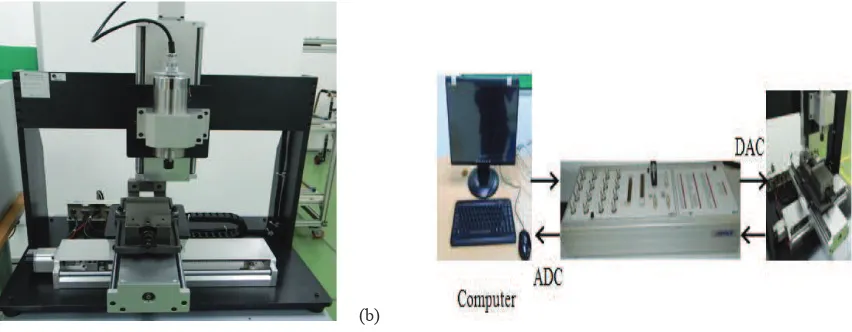
The experimental plant or test setup considered in this paper is a ballscrew drive based XY feed table of milling machine (Googol Tech GXYZ202010 series) as shown in figure 1. It is called XY Table because of the main function of X axis that move in horizontal motion and Y axis that operate in vertical motion. The dimension of the stage is 630x470x815mm (Length x Width x Height) and the weight is approximately 100kg. The plant work stage has a maximum effective travel distance of 300mm for each axis. Within the system, there is incremental rotary encoder that is attached to each axis of servo motor and is feed-backed as position signal with 2500 pulse/revolution. The axes are driven by Panasonic model MSMD 022G1U AC servo motors. The motor is coupled with high precision ball screw with a bracket and guided by sliding rod mechanism. Both axes are equipped with a 0.0005 mm encoder resolution.
(a) (b)
Fig. 1. (a) XY Milling Table (Googol Tech GXYZ202010 series) (b) Schematic diagram of experimental setup for identification of system
2.2.System Setup
In general, the experimental setup consists of 3 main elements, namely :-
x Plant (XY Table)
x Digital Signal Processing Board (dSPACE1104)
x Man Machine Interface (MMI) / Computer
The dSPACE 1104 controller board will act as a intermediate medium between plant and host computer and is used to control the position of the drives. In addition, the Matlab Simulink command that contains the tracking algorithm were uploaded to the drives from the host computer through the dSPACE to the plant for the purpose of monitoring the measured encoder signals.
3.System Identification
In the field of control systems engineering, system identification can be defined as a process of developing mathematical model that represent the dynamic behavior of the system using limited number of measurement of input and outputs[7]. During the process, the existence of noise and prior knowledge may disturb the accuracy of the mathematical model being developed. Basically, there are four basic steps in frequency domain system identification procedure[8]. The steps are as follows :-
x Step 1 : Collection of useful data (time data)
x Step 2 : Conversion from time data to frequency response function, FRF.(Non Parametric method) .
x Step 3 : Conversion from FRF to mathematical model (Parametric method).
x Step 4 : Model Validation
3.1.Collection of useful time data
First and foremost, before proceeding with the process of collecting and recording the time data, there are several questions need to be answered and decided such as selection of input signals, determination of data sampling rate, amplitude and power constraints on input and output, total time available for the experiment and availability of hardware and software for analysis purposes .
The system dynamics can be described by two single-input and single-output (SISO) models. It is decided that the selected input signals for this case is using random band limited white noise. Figure 2(a) shows the input signals which is the input voltage in unit volt that is used for the system. The reason on why this type of signal is preferred is because of the wide range of frequency content offered from this signal compared to other type of input signal like stepped sine, swept sine, multisine and impulse. On the other hand, figure 2(b) illustrates the output signals which is the position in unit millimeter. Thus, as a result, the mathematical model constructed from this signal is more robust with wide range of noise frequency. The sampling frequency used is 2000Hz, thus the sampling time is 0.0005 seconds. The total duration of the measurement is 5 minutes. A Hanning window is applied. The number of samples per window is 4096. This results a sampling resolution of 0.5 Hz. The SISO frequency response function (FRF) determined and estimated using non parametric approach via H1 estimator. H1 estimator is a classical estimator that includes the noise at the output of the system.
3.2. Conversion from time data to frequency response function, FRF (Non Parametric method)
After collecting the time data that contain input voltage (volt) with respect to time (seconds) and output position (mm) with respect to time (seconds) for both x and y-axis, The next step in System Identification is to convert from time data to frequency response function. This approach is called non parametric approach since the model created is without variable parameter or in infinite dimensional parameter spaces [9]. Other example of non-parametric model is in the type of impulse response and step response. Below is the exclusive Matlab syntax in m-file with the comment to convert from time data to frequency response function (FRF) data.
Matlab Code Comment
Ts=1/2000; % Ts = Sampling time fmin=0.1; % fmin = minimum frequency fmax=300; % fmax = maximum frequency
nrofspw=4096; % nrofspw = no. of sample per window fs=2000; % fs = Sampling frequency
p = 1; % p = no. of input q = 1; % q = no. of output x = input_sig; % x = input voltage (volt) y = output_sig; % y = output position (mm) t = Ts*[0:size(x,1)-1]'; % t = time (sec)
[Gxx,Gyy,Gyx,freq,FRF] = time2frf_h1(x,y,p,q,Ts,fmin,fmax,nrofspw)
% Gxx = input spectrum % Gyy = output spectrum
% Gyx = output-input spectrum % freq = frequency content
% FRF = frequency response function
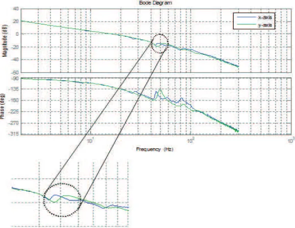
Figure 3 portrays the measured FRFs for the x and y axis.
The FRF of each axis contains an anti-resonance and resonance combination near 47 Hz based on figure 3 that has been zoomed specifically at the resonance frequency part. The factor that contributes to this condition is due to the relative motion between the base of the machine and the ground. Based on the experiment being done, study shows that a left shift in the anti-resonance and resonance frequencies when the bolts that hold the base to the ground are loosened in term of the tightness .
3.3.Conversion from FRF to mathematical model (Parametric approach)
The third step in system identification is transformation from the measured FRFs of each axis to a mathematical model called transfer function. This step is widely known as parametric approach. As the name implies, parametric approach used parameter such as poles, zeros, gain, equation of motion to represent the system. The parametric models obtained is described using a limited number of characteristic quantities called the model parameters [9]. The transfer function obtained represents the estimated model of the system. There are a lot of information in terms of dynamical behavior can be traced from the transfer function for example the order of the system (whether it is second order or higher order), system's linearity (linear or non-linear) , system's phase (minimum or non-minimum phase), system's stability and the current transient response of the system and so on. Furthermore, theoretically, there are 2 approaches for parametric estimation method, the approaches are as follows [5]:-
x Deterministic approach
x Stochastic approach
Deterministic model can be defined as a model in which every set of variable states is strictly obtained by parameters in the model and it is certain and fixed [5]. As a result, it perform consistently at every allocated time for a given set of initial conditions. In addition, deterministic model does not require statistical knowledge of the disturbances on the measured FRF. A good example of estimator that used deterministic approach are Linear least square (LLS), Non-linear least square (NLLS) and Iterative weighted linear least square estimator [10].
On the other hand, Stochastic model is a model that is probabilistic with time as independent variable and its variable states are not tabulated by a fixed and certain value but rather by probability distributions [5]. Thus, in stochastic system, there may be several possible output, each with a certain probability of occurrence for a given input. Therefore, stochastic model requires statistical knowledge of the disturbances on the measured FRF. Maximum likelihood estimator (MLE) is one example that used stochastic approach. For this experiment, deterministic approach using LLS and NLLS method were chosen. Below is the exclusively unique Matlab syntax in m-file with the comments to perform step number three.
Matlab Syntax Comment
FRF_W=ones(size(FRF))./abs(FRF); % FRF_W = frequency weighting functions n=4; % n = order of the denominator polynomial
M_mh=2; % M_mh = high order of the numerator M_ml=0; % M_ml = low order of the numerator iterno=100; % iterno = number of iterations
relvar=10^-10; % relvar = minimum relative deviation of the cost function
GN=1; % if GN==1 : Gauss Newton optimization, otherwise: Levenberg-Marquardt cORd='c'; % if 'c', continuous time model
[Bn,An,Bls,Als] = nllsfdi (FRF,freq,FRF_W,n,M_mh,M_ml,iterno,relvar,GN,cORd,fs); % Bn, An = solution after iterations
% Bls, Als = LLS solution
sys_nlls = tf (Bn, An); % To create transfer function using NLLS model sys_lls = tf (Bls, Als); % To create transfer function using LLS model
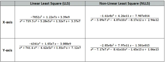
Table. 1. Estimated Model TF of the x and y axes
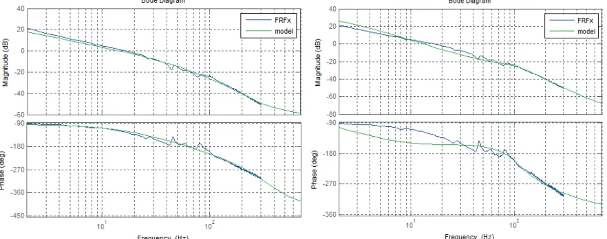
-80 Table 1 shows resulting transfer function using NLLS and LLS. Figure 4 and 5 shows the proposed model using NLLS and LLS that is being fit to the measured FRF respectively for x-axis while figure 6 and 7 for y-axis.
Fig. 4. X-axis : FRF measurement and the model using NLLS Fig. 5. X-axis : FRF measurement and the model using LLS
Fig. 6. Y-axis : FRF measurement and the model using NLLS Fig. 7. Y-axis : FRF measurement and the model using LLS
reduce the error. As a result, the NLLS method can cater both linear and non-linear system for parametric identification purposes [11-12].
3.4. Model Validation
Finally, the last step in system identification is model validation. This step is the most important step because the estimated model needs to be validated before it can be carried out throughout the whole design of the controller later on. The question is how good the model can be considered "acceptable". In the model validation stage, questions like "Does the model follow sufficiently with the time data ?", "Is the model accurate enough for my objective ?" and "Does the model represent the true system ?" need to be answered [13].
In literature there are quite few ways mentioned on how to perform the model validation procedure, they are as follows [10] :-
x Statistical Approach
(i) By comparing the feasibility of the physical parameter.
(ii) By fitting and comparing the measured FrF with the estimated model transfer function. (iii) By implementing model reduction.
(iv) By calculating the parameter confidence intervals.
(v) By simulating and comparing the system with the experimental output with the simulating output.
x Heuristic (Visual) Approach
(i) By visualizing and comparing the plot pattern of measured FrF with the model transfer function
Referring to all the techniques mentioned above, it can be seen that all the requirements have been successfully proved. First of all, in terms of the feasibility of the physical parameter, since the system have a basic structure of mass, spring and damper, thus theoretically the system should be a second order model [13]. It is proven with the estimated model. It is initially a second order model but with the addition of time delay it becomes forth order model. Secondly, based on figure 4,5,6 and 7, it is apparent that the estimated NLLS model fits better than estimated LLS model. One approach that quantifies whether the estimated model is a simple and acceptable system is to apply some model reduction or model simplification technique to it. In the case where the model is possible to be simplified without affecting the input-output properties accordingly, then the initial estimated model was "pointlessly complex"[13]. For instance, models which contain poles and zeros which are very close to each other can be cancelled out without disturbing the dynamical behavior of the system. For this case, after applying the model reduction technique (by using matlab syntax of "minreal" for the purpose of pole-zero cancellation) to the estimated model, the transfer function remain the same. It just indicates that all the poles and zeros in it are dominant and cannot be reduced [13]. The next technique is using calculation of parameter confidence interval. This technique has been discussed in previously in which the parameter confidence interval of NLLS model is better than LLS model. Therefore, in general all the requirements in model validation have been satisfied except the simulation requirement. Simulation requirement will be applied after the controller for the system has been designed.
4.Conclusion
Table 2 tabulated the overall summary of details of NLLS model transfer function for the x and y axis.
Table2. Summary of details of NLLS Model TF for the x and y axes
Parameters X - axis Y-axis
Value of time delay 0.00129 seconds 0.00138 seconds
System Linearity Linear Time Invariant (LTI) model
Resonance Frequency ~ 47 Hz
System Identification domain Frequency Domain
System Identification
Algorithm Non-parametric & Parametric
System type of phase Non-minimum Phase
Model Approach Deterministic Approach
Model Validation technique Both ( Heuristic & Statistical Technique)
System Identification is the very first process in control system design of mechatronics system. In this paper, frequency domain system identification using non parametric and parametric approach has been discussed in detail. Two types of model namely linear least square (LLS) method and non-linear least square (NLLS) methods have been used for the said purposes. Result shows that the mathematical model in transfer function form of estimated NLLS model is better than LLS model based on result during model validation stage. Graphically, the estimated NLLS model fits better than LLS model. In conclusion, the estimated model of NLLS transfer function model has been chosen to represent the system.
Acknowledgements
This research is financially supported by the Short Term Grants Scheme (PJP), Universiti Teknikal Malaysia Melaka (UTeM), with reference no. PJP/2011/FKP(24D)/S00983.
References
[1] A.M. Rankers,1997. Machine dynamics in mechatronic systems– an engineering approach, PhD Thesis, Universiteit Twente, Netherland . [2] Canudas de Wit, C., Tsiotras,P., 1999. " Dynamic Tire Friction Models for Vehicle Traction Control," Proceedings of the 38th Conference on
Decision & Control.
[3] Z. Jamaludin , 2008. Disturbance Compensation for a Machine Tools with Linear Motors, PhD Thesis, Department Wertuigkunde Katholieke Universiteit Leuven, Belgium.
[4] A.V.Kalyaev, 1959. Computing the transient response in linear systems by the method of reducing the order of the differential equations, Automat. Remote Contr. (USSR), Vol. 2, No. 1, pp. 1141-1150.
[5] Bashar H. Sader, Carl D.Sorensen, 2003. "Deterministic and stochastic dynamic modelling of continous manufacturing systems using analogies to electrical systems, " Proceedings of the 2003 Winter Simulation Conference, Vol. 2, No. 1, pp 1134-1142.
[6] R.Pintelon and J.Schoukens, 2000. System identification – a frequency domain approach, IEEE Press, New Jersey, U.S [7] J. Norton, 1986. An introduction to identification. Academic Press, ISBN 012-521730-7, London, U.K.
[8] G.C. Goodwin and R.L. Payne., 1977. Dynamic system identification, Experiment design and data analysis. Academic Press Inc., ISBN 0-12-289750-1
[9] J. Schoukens, T. Dobrowiecki, and R. Pintelon, 1998. Parametric and non- parametric identification of linear systems in the presence of nonlinear distortions, IEEE Trans. Autom.Control, pp 176-190.
[10] L.Ljung, 1999. System identification, theory for the user, Prentice-Hall, Inc, New Jersey, U.S
[11] Z. Jamaludin, H. V. Brussel and J. Swevers, 2008. Accurate Motion Control of XY High-Speed Linear Drives using Friction Model Feedforward and Cutting Forces Estimation, CIRP Annals- Manufacturing Technology, Vol. 57, Issue. 1, pp. 403-406.
[12] Z. Jamaludin, H. V. Brussel and J. Swevers, 2007. Classical Cascade and Sliding Mode Control Tracking Performances for a XY table of a High Speed Machine Tool, International Journal of Precision Technology, Vol. 1, No. 1, pp. 65-74