SUSTAINABLE ENERGY HARVESTING TECHNOLOGIES – PAST, PRESENT AND FUTURE.

(1)

SUSTAINABLE

ENERGY HARVESTING

TECHNOLOGIES – PAST,

PRESENT AND FUTURE

(2)

Sustainable Energy Harvesting Technologies – Past, Present and Future Edited by Yen Kheng Tan

Published by InTech

Janeza Trdine 9, 51000 Rijeka, Croatia

All chapters are Open Access distributed under the Creative Commons Attribution 3.0 license, which allows users to download, copy and build upon published articles even for commercial purposes, as long as the author and publisher are properly credited, which ensures maximum dissemination and a wider impact of our publications. After this work has been published by InTech, authors have the right to republish it, in whole or part, in any publication of which they are the author, and to make other personal use of the work. Any republication, referencing or personal use of the work must explicitly identify the original source.

As for readers, this license allows users to download, copy and build upon published chapters even for commercial purposes, as long as the author and publisher are properly credited, which ensures maximum dissemination and a wider impact of our publications.

Notice

Statements and opinions expressed in the chapters are these of the individual contributors and not necessarily those of the editors or publisher. No responsibility is accepted for the accuracy of information contained in the published chapters. The publisher assumes no responsibility for any damage or injury to persons or property arising out of the use of any materials, instructions, methods or ideas contained in the book.

Publishing Process Manager Vedran Greblo Technical Editor Teodora Smiljanic

Cover Designer InTech Design Team

Image Copyright olly, 2011. Used under license from Shutterstock.com

First published December, 2011 Printed in Croatia

A free online edition of this book is available at www.intechopen.com Additional hard copies can be obtained from orders@intechweb.org

Sustainable Energy Harvesting Technologies – Past, Present and Future, Edited by Yen Kheng Tan

p. cm.

(3)

(4)

(5)

Preface

In the early 21st_{century, research and development on sustainable energy harvesting} (EH) technologies have started. Since then, many EH technologies have evolved, advanced and even been successfully developed into hardware prototypes for proof of concept like Helimote, AmbiMax, et al. Researchers from all around the world are devoting their precious time and efforts into finding a realistic and novel energy harvesting solutions for sustaining the operational lifetime of low‐power electronic devices like mobile gadgets, smart wireless sensor networks, etc. Academic researchers are not the only ones focusing on sustainable EH technologies; industrial players and venture capitalists are also eyeing the EH technologies for commercialization and business development. On top of that, other disciplinary researchers like energy storage experts, smart wireless sensing and communication experts, invasive and non‐invasive biomedical experts, disaster such as forest fire management experts, etc. are also seeking for sustainable energy harvesting technologies to complement their technologies. This is based on the fact that energy harvesting is a technology that harvests freely available renewable energy from the ambient environment to recharge or put used energy back into the energy storage devices without the hassle of disrupting or even discontinuing the normal operation of the specific application.

(10)

Technologies and Future Energy Harvesting Applications; Printable, Flexible and Sustainable.

Dr. Yen Kheng Tan Energy Research Institute at Nanyang Technological University,

(11)

(12)

(13)

(14)

(15)

A Modelling Framework for Energy Harvesting

Aware Wireless Sensor Networks

Michael R. Hansen, Mikkel Koefoed Jakobsen and Jan Madsen

Technical University of Denmark, DTU Informatics, Embedded Systems Engineering Denmark

1. Introduction

A Wireless Sensor Network (WSN) is a distributed network, where a large number of computational components (also referred to as "sensor nodes" or simply "nodes") are deployed in a physical environment. Each component collects information about and offers services to its environment, e.g. environmental monitoring and control, healthcare monitoring and trafﬁc control, to name a few. The collected information is processed either at the component, in the network or at a remote location (e.g. the base station), or in any combination of these. WSNs are typically required to run unattended for very long periods of time, often several years, only powered by standard batteries. This makes energy-awareness a particular important issue when designing WSNs.

In a WSN there are two major sources of energy usage:

• Operation of a node, which includes sampling, storing and possibly processing of sensor data.

• Routing data in the network, which includes sending data sampled by the node or receiving and resending data from other nodes in the network.

Traditionally, WSN nodes have been designed as ultra low-power devices, i.e., low-power design techniques have been applied in order to achieve nodes that use very little power when operated and even less when being inactive or idle. By adjusting the duty-cycle of nodes, it is possible to ensure long periods of idle time, effectively reducing the required energy.

At the network-level nodes are equipped with low-power, low-range radios in order to use little energy, resulting in multi-hop networks in which data has to be carefully routed. A classical technique has been to ﬁnd the shortest path from any node in the network to the base station and hence, ensuring a minimum amount of energy to route data. The shortest path is illustrated in Fig. 1. Fig. 1(b) shows the circular network layout, where the base station is labelledNx. Fig. 1(a) is a bar-chart showing the distance (y-axis) from a node to the base station, the x-axis is an unfolding of the circular network, placing the base station, with a distance of zero, at both ends.

(16)

distance

Node

Nx Na Nb Nc Nd Ne Nf Ng Nx

(a)

Nx Na Nb

Nc Nd

Ne

Nf

Ng

(b)

simple distance

Fig. 1. An example network displaying the shortest distance to the base station. (a) shows each node’s distance to the base station while (b) shows the placement of each node.

the base station, resulting in a relative short lifetime of the network. To address this, energy efﬁcient algorithms, such as Bush et al. (2005); Faruque & Helmy (2003); Vergados et al. (2008), have been proposed. The aim of these approaches is to increase the lifetime of the network by distributing the data toseveralneighbours in order to minimize the energy consumption of nodes on the shortest path. However, these approaches do not consider the residual energy in the batteries. The energy-aware algorithms, such as Faruque & Helmy (2003); Hassanein & Luo (2006); Ma & Yang (2006); Mann et al. (2005); S.D. et al. (2005); Shah & Rabaey (2002); Xu et al. (2006); Zhang & Mouftah (2004), are all measuring the residual battery energy and are extending the routing algorithms to take into account the actual available energy, under the assumption that the battery energy is monotonically decreasing.

With the advances in energy harvesting technologies, energy harvesting is an attractive new source of energy to power the individual nodes of a WSN. Not only is it possible to extend the lifetime of the WSN, it may eventually be possible to run them without batteries. However, this will require that the WSN system is carefully designed to effectively use adaptive energy management, and hence, adds to the complexity of the problem. One of the key challenges is that the amount of energy being harvested over a period of time is highly unpredictable. Consider an energy harvester based on solar cells, the amount of energy being harvested, not only depends on the efﬁciency of the solar cell technology, but also on the time of day, local weather conditions (e.g., clouds), shadows from building, trees, etc.. For these conditions, the energy-aware algorithms presented above, cannot be used as they assume residual battery energy to be monotonically decreasing. A few energy harvesting aware algorithms have been proposed to address these issues, such as Islam et al. (2007); Lattanzi et al. (2007); Lin et al. (2007); Voigt et al. (2004; 2003); Zeng et al. (2006). They do not make the assumption of monotonically decreasing residual battery energy, and hence, can account for both discharging and charging the battery. Furthermore, they may estimate the future harvested energy in order to improve performance. However, these routing algorithms make certain assumptions that are not valid for multi-hop networks.

(17)

that each node have knowledge of its geographic position. Global knowledge is assumed in Lin et al. (2007).

Techniques for managing harvested energy in WSNs have been proposed, such as Corke et al. (2007); Jiang et al. (2005); Kansal et al. (2007; 2004); Moser et al. (2006); Simjee & Chou (2006). These are focussing on local energy management. In Kansal et al. (2007) they also propose a method to synchronise this power management between nodes in the network to reduce latency on routing messages to the base station. They do, however, not consider dynamic routes as such. An interesting energy harvesting aware multi-hop routing algorithm is the REAR algorithm by Hassanein & Luo (2006). It is based on ﬁnding two routes from a source to a sink (i.e. the base station), a primary and a backup route. The primary route reserve an amount of energy in each node along the path and the backup route is selected to be as disjunct from the primary route as possible. The backup route does not reserve energy along its path. If the primary route is broken (e.g. due to power loss at some node) the backup route is used until a new primary and backup route has been build from scratch by the algorithm. An attempt to deﬁne a mathematical framework for energy aware routing in multi-hop WSNs is proposed by Lin et al. (2007). The framework can handle renewable energy sources of nodes. The advantage of this framework is that WSNs can be analyzed analytically, however the algorithm relies on the ideal, but highly unrealistic assumption, that changes in nodal energy levels are broadcasted instantaneously to all other nodes. The problem with this approach is that it assumes global knowledge of the network.

The aim of this chapter is to propose a modeling framework which can be used to study energy harvesting aware routing in WSNs. The capabilities and efﬁciency of the modeling framework will be illustrated through the modeling and simulation of a distributed energy harvesting aware routing protocol, Distributed Energy Harvesting Aware Routing (DEHAR) by Jakobsen et al. (2010). In Section 2 a generic modeling framework which can be used to model and analyse a broad range of energy harvesting aware WSNs, is developed. In particular, a conceptual basis as well as an operational basis for such networks are developed. Section 3 shows the adequacy of the modeling framework by giving very natural descriptions and explanations of two energy harvesting based networks: DEHAR Jakobsen et al. (2010) and Directed Diffusion (DD) Intanagonwiwat et al. (2002). The main ideas behind routing in these networks are explained in terms of the simple network in Fig. 1. Properties of energy harvesting aware networks are analysed in Section 4 using simulation results for DEHAR and DD. These results validate that energy harvesting awareness increase the energy level in nodes, and hence, keep nodes (which otherwise would die) alive, in the sense that a complete drain of energy in critical nodes can be prevented, or at least postpone. Finally, Section 5 contains a brief summary and concluding remarks.

2. A generic modelling framework

The purpose of this section is to present a generic modelling framework which can be used to study energy-aware routing in a WSN, where the nodes of the network have an energy harvesting capability. In the next section instantiations of this generic model will be presented and experimental results through simulations are presented in Section 4.

(18)

• sensor nodes have an energy-harvesting device,

• sensor nodes are using radio-based communication, consisting of a transmitter and a receiver,

• sensor nodes are inexpensive devices with limited computational power, and

• the routing in the network adapts to dynamic changes of the available energy in the individual nodes, i.e. the routing is energy aware.

On the other hand, we will not make any particular assumptions about the kind of sensors which are used to monitor the environment.

These assumptions have consequences concerning the concepts which should be reﬂected in the modelling framework, in particular, concerning the components of a node. Some consequences are:

• A node may only be able to have a direct communication with a small subset of the other nodes, called its neighbours, due to the range of the radio communication.

• A node needs information about neighbour nodes reﬂecting their current energy levels in order to support energy-aware routing.

• A node can make immediate changes to its own state; but it can only affect the state of other nodes by use of radio communication.

• The processing in the computational units as well as the sensing, receiving and transmitting of data are energy consuming processes.

These assumptions and consequences ﬁt a broad range of WSNs.

The components of a node

A node consists of ﬁve physical components:

• Anenergy harvesterwhich can collect energy from the environment. It could be by the use of a solar panel – but the concrete energy source and harvesting device are not important in the generic setting.

• Asensorwhich is used to monitor the environment. There may be several sensors in a physical node; but we will not be concerned about concrete kinds in the generic setting and will (for simplicity) assume that one generic sensor can capture the main characteristics of a broad range of physical sensors.

• Areceiverwhich is used to get messages from the network. • Atransmitterwhich is used to send messages to the network.

• Acomputational unitwhich is used to treat sensor data, to implement the energy-aware routing algorithm, and to manage the receiving and sending of messages in the network. The model should capture that use of the sensor, receiver, transmitter and computational unit consume energy and that the only supply of energy comes from the nodes’ energy harvesters. It is therefore a delicate matter to design an energy-aware routing algorithm because a risk is that the energy required by executing the algorithm may exceed the gain by using it.

(19)

The identity of a node

We shall assume that each node has a unique identiﬁcation which is taken from a set Id of identiﬁers.

The state of a node

Thestateof a node is partitioned into acomputational stateand aphysical state. The physical state contains a model of the real energy level in the node as well as a model of the dynamics of energy devices, like, for example, a capacitor. The computational state contains an approximation of the physical energy model, including at least an approximation of the energy level. The computational state also contains routing information and an abstract view of the energy level in neighbour nodes. Furthermore, the computational state could contain information needed in the processing of observations, but we will not go into details about that part of the computational state here, as we will focus on energy harvesting and energy-aware routing.

We shall assume the existence of the following sets (or types):

• PhysicalState – which models the real physical states of the node, • Energy – which models energy levels,

• ComputationalState – which models the state in the computational unit in a node, including a model of the view of the environment (especially the neighbours) and information about the energy model and the processing of observations, and

• AbstractState – which models the abstract view of a computational state. An abstract state is intended to give a condensed version of a computational state and it can be communicated to neighbour nodes and used for energy-aware routing. It is introduced since it is too energy consuming to communicate complete state information to neighbours when radio communication is used.

The state parts of a node may change during operation. The concrete changes will not be described in the generic framework, where it is just assumed that they can be achieved using the functions speciﬁed in Fig. 2. Notice that a node can change its own state only.

Sets: PhysicalState, ComputationalState, AbstractState, and Energy

Operations:

consistent? : ComputationalState→ {true, false}

abstractView : ComputationalState→AbstractState

updateEnergyState : ComputationalState×Energy→ComputationalState

updateNeighbourView : ComputationalState×Id×AbstractState→ComputationalState updateRoutingState : ComputationalState→ComputationalState

transmitChange? : ComputationalState×ComputationalState→ {true, false}

next : ComputationalState→Id

Fig. 2. An signature for operations on the computational state

(20)

• consistent?(cs)is a predicate which is true if the computational statecsisconsistent. Since neighbour and energy information, which are used to guide the routing, are changing dynamically, a node may end up in a situation where no neighbour seems feasible as the next destination on the route to the based station. Such a situation is called inconsistent, and the predicate consistent?(cs)can test for the occurrences of such situations.

• abstractView(cs)gives the abstract view of the computational statecs. This abstract view constitutes the part of the state which is communicated to neighbours.

• updateEnergyState(cs,e)gives the computational state obtained fromcsby incorporation of the actual energy levele. The resulting computational state may be inconsistent. • updateNeighbourView(cs,id,as) gives the computational state obtained from cs by

updating the neighbour knowledge so thatasbecomes the abstract state of the neighbour nodeNid. The resulting computational state may be inconsistent.

• updateRoutingState(cs) gives the computational state obtained fromcsby updating the routing information on the basis of the energy and neighbour knowledge incsso that the resulting state is consistent.

• transmitChange?(cs,cs′) is a predicate which is true if the difference between the two computational states are so signiﬁcant that the abstract view of the "new state" should be communicated to the neighbours.

• next(cs) gives, on the basis of the computational state cs, the identiﬁer of the "best" neighbour to which observations should be transmitted.

The computation costs

Each of the above seven functions in Fig. 2 are executed on the computational unit of a node. Such an execution will consume energy and cause a change of the physical state. For simplicity, we will assume that the cost of executing the predicates consistent? and transmitChange? can be neglected or rather included in other functions, since they always incurs the same energy cost in these functions. These functions are speciﬁed in Fig. 3.

costAbstractView : PhysicalState→PhysicalState costUpdateEnergyState : PhysicalState→PhysicalState costUpdateNeighbourView : PhysicalState→PhysicalState costUpdateRoutingState : PhysicalState→PhysicalState costNext : PhysicalState→PhysicalState

The costs of the predicates consistent? and transmitChange? are assumed negligible.

Fig. 3. An signature for cost operations on the computational state

(21)

Input events of a node

The computational unit in a node can react toeventsoriginating from the energy observations on the physical state, e.g. due to the harvesting device, the sensor and the receiver. There are two energy related events, where one is concerned with the change of the physical state while the other is concerned with reading the energy level in the node. The rationale for having two events rather than a "combined" one is that the change of the physical state is a cheap operation which does not involve a reading nor any other kind of computation, whereas a reading of the energy level consumes some energy.

A sensor recording results in an observationobelonging to a set Observation of observations. An observation could be temperature measurement, a trafﬁc observation or an observation of a bird – but the concrete kind is of no importance in this generic part of the framework.

The events are described as follows:

• readEnergyEvent(e,ps), where e ∈ Energy andps ∈ PhysicalState, which is an event signalling a reading e of the energy level in the node and a resulting physical stateps, which incorporates that the reading actually consumes some energy.

• physicalStateEvent(ps), whereps∈PhysicalState is a new physical state. This event occurs when a change in the physical state is recorded. This change may, for example, be due to energy harvesting, due to a drop in energy level, or due to some other change which could be the elapse of time.

• observationEvent(o,ps), whereo∈Observation is a recorded sensor observation andps∈

PhysicalState is a physical state which incorporates the energy consumption due to the activation of the sensor.

• receiveEvent(m,ps), whereps ∈ PhysicalState and m ∈ Message, which could be an observation to be transmitted to the base station or a message describing the state of a neighbour node. Further details are given below. The receiver maintains a queue of messages. When it records a new message, that message is put into the queue. The event receiveEvent(m,ps)is offered whenmis the front element in the queue. Reacting to this event will removemfrom the queue and a new receive event will be offered as long as there are messages in the queue. It is unspeciﬁed in the generic setting whether there is a bound on the size of the queue.

Input messages

A node has a queue of messages received from the network. There are two kinds of messages:

• Observation Messages of the form obsMsg(dst,o), where dst is the identity of the next destination of the observationo∈Observation on the route to the base station.

• Neighbour Messages of the form neighbourMsg(src,as), where src is the identity of the source, i.e. the node which have sent this message, andas∈AbstractState is the contents of the message in the form of an abstract state.

(22)

Output messages and communication

A nodeNidcan use the transmitter to broadcast a messagem∈Message to the network using the commandsend

id(m). Intuitively, nodes which are within the range of the transmitter will receive this message and this may depend on the strength of the signal, it may depend on geographical positions, or on a variety of other parameters.

A model for sending and receiving messages could include a global traceof the messages send by nodes, alocal traceof messages received by the individual nodes, and a description of amedium, that determines which nodes can receive messages sent by a node Nidon the basis of the current state of the network and on the basis of the various parameters, for example, concerning geographical positions of the nodes. In instances of the generic model, such a medium must be described. In this chapter we will not be formal about network communication. A formal model of communication along the lines sketched above can be found in Mørk et al. (1996); Pilegaard et al. (2003).

The cost of sending messages

Sending a message consumes energy which is reﬂected in a change of the physical state of a node. To capture this a function

costSend : PhysicalState×Message→PhysicalState

can compute a new physical state on the basis of the current one and a broadcasted message.

An operational model of a node

During its lifetime, a node can change between two mainphases:idleandtreat message.

• The node is basically inactive in the idle phase waiting for some event to happen. It processes an incoming event and makes a phase transition.

• The node treats a single message in the treat message phase and after that it makes a transition to the idle phase.

Each phase is parameterrised by the computational statecsand the physical stateps. The state changes and phase transitions for the idle phase are given in Fig. 4. The node stays inactive in the idle phase until a event occurs.

• A physical-state event leads to a change of physical state while staying in the idle phase. • A read-energy event leads to an update of the energy and routing parts of the

computational state, and the physical state is updated by incorporation of the corresponding costs. If the changes of the computational state are insigniﬁcant then these changes are ignored (so that the nodes have a consistent knowledge of each other) and just the physical state is changed. Otherwise, the abstract view of the new computational state is computed and send to the neighbours, and both the computational and the physical states are changed.

(23)

Idleid(cs,ps) = wait

physicalStateEvent(ps′) → Idleid(cs,ps′) readEnergyEvent(e,ps′) →

let_cs′₌_{updateRoutingState}₍_{updateEnergyState}₍_cs,_e₎₎ let_ps′′₌_{costUpdateEnergyState}₍_{costUpdateRoutingState}₍_ps′₎₎ if_{transmitChange?}₍_cs,_cs′₎

then let_m₌_neighbourMsg₍_{id, abstractView}₍_cs′₎₎

send_id(_m)_{; Idle}_id(_cs′_{, costSend}(_{costAbstractView}(_ps′′)_,_m)) else_Idle

id(cs,ps′′) observationEvent(o,ps′) →

let_dst₌_next₍_cs₎ let_m₌_obsMsg₍_dst,_o₎ send

id(m); Idleid(cs, costSend(costNext(ps′),m)) receiveEvent(m,ps′) → TreatMsg_id(m,cs,ps′) Fig. 4. The Idle Phase

• A receive event indicates a pending message in the queue. That message is treated by a transition to the treat message phase.

Notice that all phase transitions from the idle phase preserve the consistency of the computational state. The only non-trivial transition to check is that from Idle_id(cs,ps) to Idleid(cs′, costSend(costAbstractView(ps′′),m). The consistency of cs′ follows since cs′ = updateRoutingState(updateEnergyState(cs,e))and updateRoutingState is expected to return a consistent computational state, at least under the assumption thatcsis consistent.

The state changes and phase transitions for the treat message phase are given in Fig. 5. In this phase the node treats a single message. After the message is treated a transition to the idle phase is performed, where it can react to further events including the receiving of another message. A message is treated as follows:

• An observation message is treated by ﬁrst checking whether this node is the destination for the message. If this is not the case, a direct transition to the idle phase is performed. Otherwise, the next destination is computed, the observation is forwarded to that destination and the physical state is updated taking the computation costs into account. The energy consumed by the test whether to discard or process a message is included in the energy consumption for receiving a message.

(24)

TreatMsg_id(m,cs,ps) = case_mof

obsMsg(dst,o) →

if_id=_dst

then let_dst′₌_next₍_cs₎ let_m′₌_obsMsg₍_dst′_,_o₎

send_id(_m′)_{; Idle}_id(_{cs, costSend}(_costNext(_ps)_,_m) else_Idle

id(cs,ps)) neighbourMsg(src,as) →

let_cs′₌_{updateNeighbourView}₍_cs,_src,_as₎ let_cs′′₌_{updateRoutingState}₍_cs′₎

let_ps′₌_{costUpdateNeighbourView}₍_{costUpdateRoutingState}₍_ps₎₎ if_{transmitChange?}₍_cs,_cs′′₎_{∨ ¬}_consistent?₍_cs′₎

then let_as′₌_abstractView₍_cs′₎ let_m=_neighbourMsg(_id,_as′) send

id(m); Idleid(cs′′, costSend(costAbstractView(ps′),m)) else_Idle_id(_cs′_,_ps′)

Fig. 5. The Treat-Message Phase

Notice that all phase transitions from the treat-message phase preserve the consistency of the computational state. The consistency preservation due to observation messages is trivial. The transition from TreatMsg_id(m,cs,ps) to Idleid(cs′′, costSend(costAbstractView(ps′),m)) preserves consistency since cs′′ is constructed by application of updateRoutingState, and this function is expected to return a consistent computational state. The transition from TreatMsg_id(m,cs,ps)to Idleid(cs′,ps′)also preserves consistency since that transition can only occur when theif_{-condition transmitChange?}₍_cs,_cs′′₎_{∨ ¬}_consistent?₍_cs′₎_{is false.}

Some of the main features of the operational descriptions in Fig. 4 and Fig. 5 are:

• A broad variety of instances of the operational descriptions can be achieved by providing different models for the sets and operations in Fig. 2 and Fig. 3. This emphasizes the generic nature of the model.

• The energy and neighbour parts of the model appear explicitly through the occurrence of the associated operations. Hence it is clear that the model reﬂects energy-aware routing using neighbour knowledge, and it is postponed to instantiations of the model to describe how it works.

• The energy cost model appears explicit in the form of the cost functions including the cost of events.

• A node will send a local view of its state to the neighbours only in the case when a significant change of the computational state has happened, which is determined by the transmitChange? predicate. The adequate definition of this predicate is a prerequisite for achieving a proper routing, as it is not difficult to imagine how it could load the network and drain the energy resources, if minimal changes to the states uncritically are broadcasted.

(25)

The generic model is based on the existence of a description of the medium through which the nodes communicates. This medium should at least determine which nodes can receive a message send by a given node in a given state. It may depend on the available energy, the geographical position, the distance from the sender, and a variety of other parameters. Furthermore, the medium may be unreliable so that messages may be lost.

The model describes the operational behavior (including the dynamics of the energy levels in the nodes) for the normal operation of a network. It would be natural to extend the model with an initialization phase where a node through repeated communications with the neighbours are building up the knowledge of the environment needed to start normal operations, i.e. making observations and routing them to the base station. We leave out this initialization part in order to focus on energy harvesting and energy-aware routing.

3. Instantiating the modelling framework

In this section it will be demonstrated that the energy-aware routing protocol DEHAR Jakobsen et al. (2010) can be considered as an instance of the generic modelling framework presented in the previous section. In order to do so, meaning must be given to the sets and operations collected in Fig. 2 and Fig. 3. This will provide a succinct presentation of the main ideas behind DEHAR. Furthermore, we will show that the DD protocol Intanagonwiwat et al. (2002) can be considered a special case of DEHAR. Concrete experiments, based on a simulation framework, depends on descriptions of the medium. This will be considered in Section 4.

3.1 A deﬁnition of the states

The abstract state comprises:

• Asimple distance d ∈ R≥0to the base station. This is described by a non-negative real number, where larger number means longer distance.

• Anenergy-aware adjustment a∈ R≥0of the distance for the route to the base station, where a larger distance means less energy is available.

Hence an abstract state is a pair(d,a)∈AbstractState, where

AbstractState=R≥0× R≥0

For an abstract state(d,a), we call dist(d,a) =d+atheenergy-adjusted distance.

The computational state comprises:

• Asimple distance d∈ R≥0to the base station, like the simple distance of an abstract state. • Anenergy level e∈Energy.

• Anenergy-faithful adjustment f ∈ R≥0capturing energy deﬁciencies along the route to the base station.

(26)

Hence a computational state is a 4-tuple(d,e,f,nt)∈ComputationalState, where

ComputationalState=R≥0×Energy× R≥0×(Id→AbstractState)

We shall assume that there is a function energyToDist : Energy→ R≥0that converts energy to a distance so that less energy means longer distance.

The value energyToDist(e)provides a local adjustment of the distance to the base station by just taking the energy level in the node into account. The intension with the energy-faithful adjustment is that the energy deﬁciencies along the route to the base station is taken into account, and the energy-faithful part is maintained by the use of the neighbour messages.

Theenergy adjustment of a computational state is the sum of the converted energy and the energy-faithful adjustment:

adjust(d,e,f,nt) =energyToDist(e) +f

and the energy-adjusted distance of a computational state is:

dist(d,e,f,nt) =d+adjust(d,e,f,nt) =d+energyToDist(e) +f

where we overload the dist function to be applied to both abstract and computational states. Furthermore, dist(id),id∈Id, is the distance of the abstract state of the neighbour nodeNid. The function next : ComputationalState→Id should give the neighbour with the shortest energy-adjusted distance to the base station, i.e. the "best" neighbour to forward an observation. Hence, next(d,e,f,nt)is the identityidof the entry(id,as)∈ntwith the smallest energy-adjusted distance to the base station, i.e. the smallest dist(as). If several neighbours have the smallest distance an arbitrary one is chosen.

A computational statecsis consistent if next(cs)has a smaller energy-adjusted distance than cs, i.e. dist(cs)>_dist₍_next₍_cs₎₎_{, hence}

consistent?(cs) =dist(cs)>dist(next(cs))

A node with a consistent computational state has a neighbour to which it can forward an observation. But if the state is inconsistent, then all neighbours have longer energy-adjusted distances to the base station and it does not make sense to forward an observation to any of these neighbours.

(27)

dist

(

cs

)

Node

(a) Nx Na Nb Nc Nd Ne Nf Ng (b)

simple distance:d

energy deﬁcit: energyToDist(e)

Fig. 6. The example from Fig. 1 with an energy adjustment forNedue to shaded region shown to the right.

dist

(

cs

)

Node

simple distance:d

energy deﬁcit: energyToDist(e)

Fig. 7. Revised example with an inconsistent node:Ne.

Energy-faithful adjustments can be used to cope with inconsistent nodes. By adding such adjustments to the "problematic nodes" inconsistencies may be avoided. This is shown in Fig. 8, where energy-faithful adjustments (f) have been added toNeandNf. Every node is consistent, and there is a natural route from every node to the base station. FromNfthere are actually two possible routes.

dist

(

cs

)

Node

simple distance:d

energy deﬁcit: energyToDist(e) energy-faithful adjustment:f

Fig. 8. A with consistent nodes using energy-faithful adjustments

The physical state comprises:

• The stored energye∈Energy.

• A model of the energy harvester. In the DEHAR case it is a solar panel, which is modelled by a functionP(t)describing the effect of the solar insolation at timet.

(28)

• A model of the computational unit. This model must define the costs of the computational operations by providing definitions for the cost functions in Fig. 3. A simple way of doing this is to count the instructions needed for executing the individual functions, and multiply it with the energy needed per instruction. The model can be more fine grained by taking different modes of the processing unit into account.

• A model of the transmitter. This model must give a deﬁnition of the cost function: costSend : PhysicalState×Message → PhysicalState. In the DEHAR case the cost of sending is a simple linear function in the size of the message.

• A model of the receiver. This model must explain the cost of a receive event receiveEvent(m,ps). This involves the cost of receiving the messagemand it must also take the intervals into account when the receiver isidle listening, i.e. it actively listens for incoming messages. Thuspsshould reﬂect the full energy consumption of the receiver since the last receive event.

• A model of the sensor. This model must explain the cost of an observation event observationEvent(o,ps). This involves the cost of sensing o andps should reﬂect this energy consumption.

The model should also describe two transitions of the physical state which relate to the two events physicalStateEvent(ps)and readEnergyEvent(e,ps).

The transition related to a physicalStateEvent must take into account at least the dynamics of the energy harvester, the dynamics of the energy store, the time the computational unit spent in the idle phase, and the time elapsed since the last physical state event. For example the new stored energye′in the physical state at timet′is given by:

e′=e+

_t′

t P(t)dt wheretis the time where the old energyewas stored.

The transition related to a readEnergyEvent(e,ps)must take into account at least the cost of reading the energy.

3.2 Deﬁnition of operations

The function for extracting the abstract view is deﬁned by:

abstractView(d,e,f,nt) = (d, adjust(d,e,f,nt))

Notice that the distance to the base station is preserved by the conversion from a computational state to an abstract one:

dist(d,e,f,nt) =dist(abstractView(d,e,f,nt))

The deﬁnitions of the functions for updating the energy state and the neighbour view are simple:

updateEnergyState((d,e,f,nt),e′) = (d,e′,f,nt)

(29)

where update(nt,id,as) gives the neighbour table obtained from ntby mapping id to the abstract stateas. These two operations may transform a consistent state into an inconsistent one.

The function updateRoutingState(d,e,f,nt) must update the energy adjustment of a computational state in order to arrive at a consistent one. If the state is consistent even when f =0 then no adjustment is necessary. Otherwise, an adjustment is made so that the distance of the computational state becomesKlarger than the distance of its "best" neighbour (given by the next function):

updateRoutingState(d,e,f,nt) = if_consistent?₍_d,_{e, 0,}_nt₎ then(_d,_{e, 0,}_nt)

else let_distNext₌_dist₍_next₍_d,_e,_f_,_nt₎₎

(d,e,K+distNext−(d+energyToDist(e)),nt)

whereK>_{0 is a constant used to enforce a consistent computational state.}

The energy adjustment in theelse_{-branch of this function has the effect that the node becomes} less attractive to forward messages to in the case of an energy drop in the node or in the best neighbour.

The function transmitChange?(cs,cs′) is a predicate which is true when a change of the computational state fromcstocs′is significant enough to be communicated to the neighbours. This is the case if the change reflects a significant change in distance to base station, where significant in this case means larger than some constantK_change∈ R≥0.

Hence, the function can be deﬁned as follows:

transmitChange?(cs,cs′) =|dist(cs)−dist(cs′)|>_K_change

A simple check of the operational descriptions in Fig. 4 and Fig. 5 shows that the new computational state used as argument to transmitChange? (cs′in Fig. 4 andcs′′in Fig. 5) must be consistent as it is created using updateRoutingState. Hence it is just necessary to deﬁne transmitChange? for consistent computational states.

Directed Diffusion – another instantiation of the generic framework

It should be noticed that the routing algorithm DD Intanagonwiwat et al. (2002) is a simple instance of the generic framework, which can be achieved by simplifying the DEHAR instance so that

• the simple distance is the number of hops to the based station (as for DEHAR) and • the energy is assumed perfect and hence the adjustments have no effect (are 0).

Hence DD do not support any kind of energy-aware routing.

Actually, it is the algorithm behind DD which is used to initialize the simple distances of nodes in the DEHAR algorithm.

(30)

harvesting capability, but the routing is static in the sense that an observation is always transmitted along the path with the smallest number of hops to the base station. Energy harvesting aware routing algorithms will not necessarily choose this shortest path, since problematic low-energy nodes should be avoided in order to keep all nodes “alive” as long as possible. Therefore, the total energy consumption in a DD based network should be smaller than the total energy consumption of any energy harvesting aware network (due to longer pathes in the latter). On the other hand, energy harvesting awareness can spare low-energy nodes, and there are two important consequences of this:

• A drain of low-energy nodes can be avoided or at least postponed. With regard to this aspect DD should perform worse since these nodes are not spared at all in the routing. • The total energy stored in a network should exceed that of a corresponding DD based

network, since messages are transmitted through nodes with good energy harvesting capability. The reason for this is that low-energy nodes get a chance to recover and that transmissions through high-energy nodes, with a full energy storage, are close to be “free of charge” since there would be almost no storage available for harvested energy in these high-energy nodes.

4. Results from simulation of the model

In this section we will study the properties of the energy harvesting aware routing algorithm DEHAR by analyzing results Jakobsen et al. (2010) of a simulator implementing the DEHAR and DD algorithms. The simulator is a custom-made simulator Jakobsen (2008) implemented in the language Java. It can be configured through a comprehensive xml configuration file which includes the network layout, environmental properties (insolation, shadows, etc.) and properties of nodes (such as processor states, radio model, and frequency of observations). The simulator features a classic event driven engine. The simulator produces a trace of observations of the nodes, including energy levels, activity of devices, and environmental properties

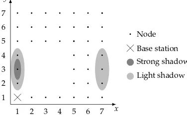
The considered network is given in Fig. 9. The network has one very problematic node, due to a strong shadow, at coordinate(1, 3), and ﬁve nodes with potential problems due to light shadows. We will analyse the ability of the routing algorithms to cope with these problematic nodes using simulations.

1 1

2 2

3 3

4 4

5 5

6 6

7 7

y

x

Node

Base station Strong shadow

[image:30.482.144.332.449.567.2]

Light shadow

(31)

The medium and the physical setting must be deﬁned for the experiments. It is assumed that a node can communicate with its immediate horizontal and vertical neighbour, i.e. the radio range is 1. Two experimentsS1 andS2 are conducted, one with a low and another with a high rate of conducted observations. Table 1 shows the parameters that are used in the presented simulations. Only the observation rate is changed between the two simulations.

S1 S2 unit

Radio

Range 1 1

Transmit power 50 50 mW Idle listening power 5.5 5.5 mW

Bandwidth 45 45 kb/s

Processor

Sleep Power 1 1 µW

ActiveFrequency 1 1 MHz

Power 10 10 µW

Battery Capacity 4 4 kJ

Solar panel Efﬁciency 6.25 6.25 %

Area 12.5 12.5 cm2

Application parameters Observation rate ₉₀₀1 ₆₀1 sec−1 Routing parameters Sense rate ₁₈₀₀1 ₁₈₀₀1 sec−1

Table 1. Parameters used in simulations.

The energy model is based on real insolation data for a two-weeks period. The data is repeated in simulations over longer periods. To emphasize the effect of the DEHAR algorithm, the insolation pattern have been idealised to either full noon or midnight, i.e. 12 hours of light and 12 hours of darkness. The insolation data is suitably scaled for individual nodes to achieve the shadow effect shown in Fig. 9.

Energy awareness makes a difference

A 30 day view of the simulationsS1with the low observation rate is shown in Fig. 10. The figure shows the energy available in the worst node with minimum energy in the network. The two algorithms cannot be distinguished the first five days. Thereafter, the energy aware routing starts and DEHAR stabilises at a high level where no node is in any danger of being drained for energy. In the DD case, the energy of worst node is steadily drained at a (rather) constant rate and in an foreseeable future it will stop working.

Energy awareness consumes and stores more energy

The total power consumed and the average energy stored per node in the network are monitored for the same simulations as in Fig. 10. These results are shown for the ﬁrst 10 days of simulated time in Fig. 11.

The day cycle is clearly visible in Fig. 11(a) where the nodes recharge during day and discharge during night. The first five days of simulation does not show any significant difference between DEHAR and DD. During the last five days the DEHAR algorithm makes the network able to harvest and store more energy.

(32)

DEHAR minimum

DD minimum

Time (h)

%

of

full

char

ge

DD DEHAR

0 48 96 144 192 240 288 336 384 432 480 528 576 624 672 72091

92 93 94 95 96 97 98 99 100

Fig. 10. Results of simulationsS1for a 30 day simulation. This graph shows the minimum energy in any node in the network.

signiﬁcantly more energy than the DD algorithm. By looking at the third graph (Fig. 11(c)) which shows the difference in total network energy consumption, it can be conﬁrmed. This extra energy consumption arises from observation packages that travel along longer routes in the network, because the DEHAR algorithm have detected a lower amount of stored energy in some nodes.

Even though the DEHAR consumes more energy due to the longer routes, it can store more energy on average in the nodes. The reason for this is that the extra energy consumption of DEHAR is taken from nodes that are able to recharge fully during daytime. This can be seen in Fig. 11(b) (in the blow-up) at the beginning of day 5 (120h), where the graph shows a sudden rise.

After a short while, the network with the DD algorithm is able to harvest energy at a greater rate than DEHAR. This is due to the fact that the majority of the nodes in the DEHAR network are fully charged. The key point at this time is that the DD algorithm does not allow the network to harvest as much energy as the DEHAR algorithm. This can also be seen through the rest of the daylight during day 5, where the DEHAR network is able to harvest energy at a higher rate than the DD network.

Finally, during night, the DEHAR network again shows a higher energy consumption than the DD network. Hence the graph shows a slow decline.

Increasing the rate of observations costs

The next simulations (S2) have an increased rate of observations and thus an increased radio trafﬁc in the network. The effect of the increased data rate is primarily that the network consumes more power. This extra power consumption speeds up the time from the start of the simulation until the network ﬁnds the alternate routing pattern compared to theS1 simulations.

(33)

DEHAR

DD

Time (h)

%

of

full

char

ge

DD DEHAR

0 24 48 72 96 120 144 168 192 216 24099.75

99.80 99.85 99.90 99.95 100.00

(a) Average energy in nodes for each simulation ofS1.

3x zoom

Time (h)

%

of

full

char

ge

0 24 48 72 96 120 144 168 192 216 240-0.005

0 0.005 0.010 0.015 0.020 0.025 0.030

(b) Difference in the average energy in nodes for simulations inS1. Given that the two curves in Fig. 11(a) are characterised by the functionsf_DEHAR(t)andf_DD(t), then the curve in this ﬁgure is characterised by

f_DEHAR(t)−f_DD(t).

Time (h)

Power

(

µ

W)

0 24 48 72 96 120 144 168 192 216 240 0

0.05 0.10 0.15 0.20 0.25 0.30

(c) Surplus energy consumption by DEHAR compared with DD for simulations inS1.

(34)

EARP minimum

DD minimum

Time (h)

%

of

full

char

ge

DD DEHAR

0 24 48 72 96 120 144 168 192 216 24020

30 40 50 60 70 80 90 100

Fig. 12. Minimum energy in any node of the simulations inS2. The day cycle is barely visible due to the compressed y-scale, compared to the simulationsS1.

The routing trend of the DEHAR algorithm is the same in the simulationsS1andS2. The only difference is that the DEHAR algorithm ﬁnds this alternative routing pattern faster inS2than inS1.

The energy statistics of the node covered by the strongest shadow (at coordinate (1,3)) can be analysed. A graph of the energy level of this node will look similar to Fig. 12 and (in this simulation) it stabilises at precisely the same energy level. This show that the energy it can harvest closely matches the energy it needs to perform routing updates and performing observations (i.e. refraining from routing other nodes observations).

5. Conclusion

We have presented a new modelling framework aimed at describing and analysing wireless sensor networks with energy harvesting capabilities. The framework comprises of a conceptual basis and an operational basis, which were used to describe and explain two wireless sensor networks with energy harvesting capabilities. One of these network models is based on DD, i.e. it supports energy harvesting; but the routing is not energy aware, as it just forwards observations to the base station along statically defined shortest pathes. The other network model is based on the energy harvesting aware routing protocol DEHAR. Both of these networks were given natural explanations using the concepts of the modelling framework, and this gives a first weak validation of the adequacy of the framework. More experiments are, of course, needed for a thorough validation. Simulation results show that energy awareness of DEHAR-based networks can significantly extend the lifetime of nodes and it significantly improves the energy stored in the network, compared with a network like DD, with no energy aware routing.

There are several natural extension of this work.

(35)

The generic framework may be instantiated in ways which will not be beneﬁcial for the energy situation in the network. It is desirable and challenging to establish conditions which instantiations should satisfy in order to deﬁne an adequate energy harvesting aware network.

Another natural development would be to implement a platform for the modelling framework. The formalized parts of the framework provide good bases for such an implementation; but further formalization concerning the network communication and the medium should be considered prior to an implementation.

6. Acknowledgment

This research has partially been funded by the SYSMODEL project (ARTEMIS JU 100035) and by the IDEA4CPS project granted by the Danish Research Foundation for Basic Research.

7. References

Bush, L. A., Carothers, C. D. & Szymanski, B. K. (2005). Algorithm for Optimizing Energy Use and Path Resilience in Sensor Networks,Wireless Sensor Networks, 2005. Proc. of the Second European Workshop on, pp. 391 – 396.

Corke, P., Valencia, P., Sikka, P., Wark, T. & Overs, L. (2007). Long-duration solar-powered wireless sensor networks, Proc. of the 4th workshop on Embedded networked sensors, ACM, pp. 33–37.

Faruque, J. & Helmy, A. (2003). Gradient-based routing in sensor networks,SIGMOBILE Mob. Comput. Commun. Rev.7(4): 50–52.

Hassanein, H. & Luo, J. (2006). Reliable Energy Aware Routing in Wireless Sensor Networks, Dependability and Security in Sensor Networks and Systems, 2006, IEEE, pp. 54–64. Intanagonwiwat, C., Govindan, R., Estrin, D., Heidemann, J. & Silva, F. (2002). Directed

Diffusion for Wireless Sensor Networking, IEEE/ACM Transactions on Networking 11(1): 2–16.

Islam, J., Islam, M. & Islam, N. (2007). A-sLEACH: An Advanced Solar Aware Leach Protocol for Energy Efﬁcient Routing in Wireless Sensor Networks,International Conference on Networking0: 4.

Jakobsen, M. K. (2008).Energy harvesting aware routing and scheduling in wireless sensor networks, Master’s thesis, Technical University of Denmark, Department of Informatics and Mathematical Modeling.

Jakobsen, M. K., Madsen, J. & Hansen, M. R. (2010). DEHAR: A distributed energy harvesting aware routing algorithm for ad-hoc multi-hop wireless sensor networks, World of Wireless Mobile and Multimedia Networks (WoWMoM), 2010 IEEE International Symposium on a, pp. 1 –9.

Jiang, X., Polastre, J. & Culler, D. (2005). Perpetual environmentally powered sensor networks, Information Processing in Sensor Networks, 2005. IPSN 2005. Fourth International Symposium on, IEEE Press, pp. 463 – 468.

Kansal, A., Hsu, J., Zahedi, S. & Srivastava, M. B. (2007). Power management in energy harvesting sensor networks,ACM Trans. Embed. Comput. Syst.6(4): 32.

(36)

Lattanzi, E., Regini, E., Acquaviva, A. & Bogliolo, A. (2007). Energetic sustainability of routing algorithms for energy-harvesting wireless sensor networks, Comput. Commun.30(14-15): 2976–2986.

Lin, L., Shroff, N. B. & Srikant, R. (2007). Asymptotically optimal energy-aware routing for multihop wireless networks with renewable energy sources,IEEE/ACM Transactions on Networking15(5): 1021–1034.

Ma, C. & Yang, Y. (2006). Battery-aware routing for streaming data transmissions in wireless sensor networks,Mob. Netw. Appl.11(5): 757–767.

Mann, R. P., Namuduri, K. R. & Pendse, R. (2005). Energy-Aware Routing Protocol for Ad Hoc Wireless Sensor Networks, EURASIP Journal on Wireless Communications and Networking2005(5): 635–644.

Mørk, S., Godskesen, J., Hansen, M. R. & Sharp, R. (1996). A timed semantics for sdl, in R. Gotzhein & J. Bredereke (eds),Formal Description Techniques IX: Theory, application and tools, Chapman & Hall, pp. 295–309.

Moser, C., Thiele, L., Benini, L. & Brunelli, D. (2006). Real-Time Scheduling with Regenerative Energy,Proc. of the 18th Euromicro Conf. on Real-Time Systems, IEEE Computer Society, pp. 261–270.

Pilegaard, H., Hansen, M. R. & Sharp, R. (2003). An approach to analyzing availability properties of security protocols,Nordic Journal of Computing10: 337–373.

S.D., M., D.C.F., M., R.I., B. & A.O., F. (2005). A centralized energy-efﬁcient routing protocol for wireless sensor networks,IEEE Communications Magazine43(3): S8–13.

Shah, R. C. & Rabaey, J. M. (2002). Energy aware routing for low energy ad hoc sensor networks,Wireless Communications and Networking Conf., 2002, Vol. 1, IEEE, pp. 350 – 355.

Simjee, F. & Chou, P. H. (2006). Everlast: long-life, supercapacitor-operated wireless sensor node,Proc. of the 2006 intl. symposium on Low power electronics and design, ACM Press, pp. 197–202.

Vergados, D. J., Pantazis, N. A. & Vergados, D. D. (2008). Energy-efﬁcient route selection strategies for wireless sensor networks,Mob. Netw. Appl.13(3-4): 285–296.

Voigt, T., Dunkels, A., Alonso, J., Ritter, H. & Schiller, J. (2004). Solar-aware clustering in wireless sensor networks,IEEE Symp. on Computers and Communications1: 238–243. Voigt, T., Ritter, H. & Schiller, J. (2003). Solar-aware Routing in Wireless Sensor Networks,Intl.

Workshop on Personal Wireless Communications, Springer, pp. 847–852.

Xu, J., Peric, B. & Vojcic, B. (2006). Performance of energy-aware and link-adaptive routing metrics for ultra wideband sensor networks,Mob. Netw. Appl.11(4): 509–519. Zeng, K., Ren, K., Lou, W. & Moran, P. J. (2006). Energy-aware geographic routing in lossy

wireless sensor networks with environmental energy supply,Proc. of the 3rd intl. conf. on Quality of service in heterogeneous wired/wireless networks, ACM Press, p. 8.

(37)

Vibration Energy Harvesting: Machinery

Vibration, Human Movement and

Flow Induced Vibration

Dibin Zhu

University of Southampton

UK

1. Introduction

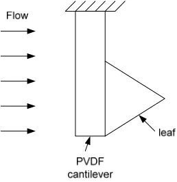
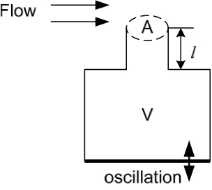
With the development of low power electronics and energy harvesting technology, self-powered systems have become a research hotspot over the last decade. The main advantage of self-powered systems is that they require minimum maintenance which makes them to be deployed in large scale or previously inaccessible locations. Therefore, the target of energy harvesting is to power autonomous ‘fit and forget’ electronic systems over their lifetime. Some possible alternative energy sources include photonic energy (Norman, 2007), thermal energy (Huesgen et al., 2008) and mechanical energy (Beeby et al., 2006). Among these sources, photonic energy has already been widely used in power supplies. Solar cells provide excellent power density. However, energy harvesting using light sources restricts the working environment of electronic systems. Such systems cannot work normally in low light or dirty conditions. Thermal energy can be converted to electrical energy by the Seebeck effect while working environment for thermo-powered systems is also limited. Mechanical energy can be found in instances where thermal or photonic energy is not suitable, which makes extracting energy from mechanical energy an attractive approach for powering electronic systems. The source of mechanical energy can be a vibrating structure, a moving human body or air/water flow induced vibration. The frequency of the mechanical excitation depends on the source: less than 10Hz for human movements and typically over 30Hz for machinery vibrations (Roundy et al., 2003). In this chapter, energy harvesting from various vibration sources will be reviewed. In section 2, energy harvesting from machinery vibration will be introduced. A general model of vibration energy harvester is presented first followed by introduction of three main transduction mechanisms, i.e. electromagnetic, piezoelectric and electrostatic transducers. In addition, vibration energy harvesters with frequency tunability and wide bandwidth will be discussed. In section 3, energy harvesting from human movement will be introduced. In section 4, energy harvesting from flow induced vibration (FIV) will be discussed. Three types of such generators will be introduced, i.e. energy harvesting from vortex-induced vibration (VIV), fluttering energy harvesters and Helmholtz resonator. Conclusions will be given in section 5.

2. Energy harvesting from machinery vibration

(38)

[image:38.482.114.373.172.293.2]

linear energy harvesters. A generic model for linear vibration energy harvesters was first introduced by Williams & Yates (Williams & Yates, 1996) as shown in Fig. 1. The system consists of an inertial mass, m, that is connected to a housing with a spring, k, and a damper, b. The damper has two parts, one is the mechanical damping and the other is the electrical damping which represents the transduction mechanism. When an energy harvester vibrates on the vibration source, the inertial mass moves out of phase with the energy harvester’s housing. There is either a relative displacement between the mass and the housing or mechanical strain.

Fig. 1. Generic model of linear vibration energy harvesters

In Fig. 1, x is the absolute displacement of the inertial mass, y is the displacement of the housing and z is the relative motion of the mass with respect to the housing. Electrical energy can then be extracted via certain transduction mechanisms by exploiting either displacement or strain. The average power available for vibration energy harvester, including power delivered to electrical loads and power wasted in the mechanical damping, is (Williams & Yates, 1996):

 

2 2 2 3 3 2 2 1 _⎥ ⎦ ⎤ ⎢ ⎣ ⎡  ⎥ ⎥ ⎦ ⎤ ⎢ ⎢ ⎣ ⎡           r T r r TY m P ωω ζ ωω ω ωω ζ

ω (1)

where is the total damping, Y is the displacement of the housing and ωr is the resonant

frequency.

Each linear energy harvester has a fixed resonant frequency and is always designed to have a high quality (Q) factor. Therefore, a maximum output power can be achieved when the resonant frequency of the generator matches the ambient vibration frequency as:

T r mY P ζω 4 3 2

 (2)

(39)

r

ma P

ζω 4

2

 (3)

where a Y ω2 is the excitation acceleration. Eq. 3 shows that output power of a vibration energy harvester is proportional to mass and excitation acceleration squared and inversely proportional to its resonant frequency and damping.

When the resonant frequency of the energy harvester does not match the ambient frequency, the output power level will decrease dramatically. This drawback severely restricts the development of linear energy harvesters. To date, there are generally two possible solutions to this problem (Zhu et al., 2010a). The first is to tune the resonant frequency of a single generator periodically so that it matches the frequency of ambient vibration at all times and the second solution is to widen the bandwidth of the generator. These issues will be discussed in later sections.

There are three commonly used transduction mechanisms, i.e. electromagnetic, piezoelectric and electrostatic. Relative displacement is used in electromagnetic and electrostatic transducers while strain is exploited in piezoelectric transducer to generate electrical energy. Details of these three transducers will be presented in the next few sections.

2.1 Electromagnetic vibration energy harvesters

Electromagnetic induction is based on Faraday's Law which states that “an electrical current will be induced in any closed circuit when the magnetic flux through a surface bounded by the conductor changes“. This applies whether the magnetic field changes in strength or the conductor is moved through it. In electromagnetic energy harvesters, permanent magnets are normally used to produce strong magnetic field and coils are used as the conductor. Either the permanent magnet or the coil is fixed to the frame while the other is attached to the inertial mass. In most cases, the coil is fixed while the magnet is mobile as the coil is fragile compared to the magnet and static coil can increase lifetime of the device. Ambient vibration results in the relative displacement between the magnet and the coil, which generates electrical energy. According to the Faraday’s Law, the induced voltage, also known as electromotive force (e.m.f), is proportional to the strength of the magnetic field, the velocity of the relative motion and the number of turns of the coil.

Generally, there are two types of electromagnetic energy harvesters in terms of the relative displacement. In the first type as shown in Fig. 2(a), there is lateral movement between the magnet and the coil. The magnetic field cut by the coil varies with the relative movement between the magnet and the coil. In the second type as shown in Fig. 2(b), the magnet moves in and out of the coil. The magnetic field cut by the coil varies with the distance between the coil and the magnet. In contrast, the first type is more common as it is able to provide better electromagnetic coupling.

(40)

[image:40.482.75.407.98.177.2] [image:40.482.97.389.257.464.2]

(a) (b) Fig. 2. Two types of electromagnetic energy harvesters

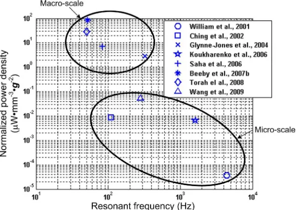
Fig. 3 compares normalized power density of some reported electromagnetic vibration energy harvesters. It is clear that power density of macro-scaled electromagnetic vibration energy harvesters is much higher than that of micro-scaled devices. This proves analytical results presented by Beeby et al (2007a).

Fig. 3. Comparisons of normalized power density of some existing electromagnetic vibration energy harvesters

2.2 Piezoelectric vibration energy harvesters

(41)

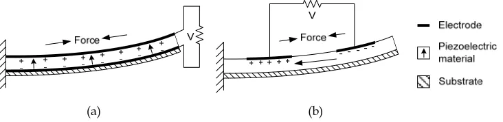
shown in Fig. 4. In d31 mode, a lateral force is applied in the direction perpendicular to the polarization direction, an example of which is a bending beam that has electrodes on its top and bottom surfaces as in Fig. 4(a). In d33 mode, force applied is in the same direction as the polarization direction, an example of which is a bending beam that has all electrodes on its top surfaces as in Fig. 4(b). Although piezoelectric materials in d31 mode normally have a lower coupling coefficients than in d33 mode, d31 mode is more commonly used (Anton and Sodano, 2007). This is because when a cantilever or a double-clamped beam (two typical structures in vibration energy harvesters) bends, more lateral stress is produced than vertical stress, which makes it easier to couple in d31 mode.

[image:41.482.59.425.193.282.2]

(a) (b)

Fig. 4. Two types of piezoelectric energy harvesters (a) d31 mode (b) d33 mode

Piezoelectric energy harvesters have high output voltage but low current level. They have simple structures, which makes them compatible with MEMS. However, most piezoelectric materials have poor mechanical properties. Therefore, lifetime is a big concern for piezoelectric energy harvesters. Furthermore, piezoelectric energy harvesters normally have very high output impedance, which makes it difficult to couple with follow-on electronics efficiently. Commonly used materials for piezoelectric energy harvesting are BaTiO3, PZT-5A, PZT-5H, polyvinylidene fluoride (PVDF) (Anton & Sodano, 2007). In theory, with the same dimensions, piezoelectric energy harvesters using PZT-5A has the most amount of output power (Zhu & Beeby, 2011).

Fig. 5 compares normalized power density of some reported piezoelectric vibration energy harvesters. It is found that micro-scaled piezoelectric energy harvesters have a greater power density than macro-scale device. However, due to size constraints in micro-scaled energy harvesters, the absolute amount of output power produced by the micro-scaled energy harvesters is much lower than that produced by the macro-scaled generators. Therefore, unless the piezoelectric energy harvesters are to be integrated into a micromechanical or microelectronic system, macro-scaled piezoelectric generators are preferred. Normalized power density of piezoelectric energy harvesters is about the same level as that of electromagnetic energy harvesters.

(42)

Fig. 5. Comparisons of normalized power density of some existing piezoelectric vibration energy harvesters

2.3 Electrostatic vibration energy harvesters

Electrostatic energy harvesters are based on variable capacitors. There are two sets of electrodes in the variable capacitor. One set of electrodes are fixed on the housing while the other set of electrodes are attached to the inertial mass. Mechanical vibration drives the movable electrodes to move with respect to the fixed electrodes, which changes the capacitance. The capacitance varies between maximum and minimum value. If the charge on the capacitor is constrained, charge will move from the capacitor to a storage device or to the load as the capacitance decreases. Thus, mechanical energy is converted to electrical energy. Electrostatic energy harvesters can be classified into three types as shown in Fig. 6, i.e. In-Plane Overlap which varies the overlap area between electrodes, In-Plane Gap Closing which varies the gap between electrodes and Out-of-Plane Gap which varies the gap between two large electrode plates.

(a) (b) (c)

(43)

Electrostatic energy harvesters have high output voltage level and low output current. As they have variable capacitor structures that are commonly used in MEMS devices, it is easy to integrate electrostatic energy harvesters with MEMS fabrication process. However, mechanical constraints are needed in electrostatic energy harvesting. External voltage source or pre-charged electrets is also necessary. Furthermore, electrostatic energy harvesters also have high output impedance.

Fig. 7 compares normalized power density of some reported electrostatic vibration energy harvesters. Normalized power density of electrostatic energy harvesters is much lower than that of the other two types of vibration energy harvesters. However, dimensions of electrostatic energy harvesters are normally small which can be easily integrated into chip-level systems.

Fig. 7. Comparisons of normalized power density of some existing electrostatic vibration energy harvesters

2.4 Tunable vibration energy harvesters

As mentioned earlier, most vibration energy harvesters are linear devices. Each device has only one resonant frequency. When the ambient vibration frequency does not match the resonant frequency, output of the energy harvester can be reduced significantly. One potential method to overcome this drawback is to tune the resonant frequency of the energy harvester so that it can match the ambient vibration frequency at all time.

(44)

once the resonant f