Faculty of Mechanical Engineering
A CORRECTED MODEL OF
STATISTICAL ENERGY ANALYSIS (SEA)
IN A NON-REVERBERANT ACOUSTIC SPACE
Al Munawir
Master of Science in Mechanical Engineering
A CORRECTED MODEL OF
STATISTICAL ENERGY ANALYSIS (SEA) IN A NON-REVERBERANT ACOUSTIC SPACE
AL MUNAWIR
A thesis submitted
in fulfillment of the requirements for the degree of Master of Science in Mechanical Engineering
Faculty of Mechanical Engineering
UNIVERSITI TEKNIKAL MALAYSIA MELAKA
DECLARATION
I declare that this thesis entitled ”A Corrected Model of Statistical Energy Analysis (SEA) In
A Non-Reverberant Acoustic Space” is the result of my own research except as cited in the
references. The Thesis has not been accepted for any degree and is not currently submitted
in candidate of any other degree.
Signature : ...
Name : ...
APPROVAL
I hereby declare that I have read this thesis and in my opinion this thesis is sufficient in terms
of scope and quality for the award of Master of Science in Mechanical Engineering
Signature : ...
Supervisor Name : ...
DEDICATION
ABSTRACT
Statistical Energy Analysis (SEA) is a well-known method to analyze the flow of acoustic
and vibration energy in a complex structure. The method is based on the power balance
equa-tion where energy in the divided subsystems must be reverberant. This study investigates the
application of SEA model in a non-reverberant acoustic space where the direct field
compo-nent dominates the total sound field rather than a diffuse field in a reverberant space. Here, a
corrected SEA model is proposed where the direct field component in the energy is removed
and the power injected in the subsystem considers only the remaining power after the loss at
first reflection. To validate the model, a measurement was first conducted in a box divided
into two rooms where the condition of reverberant and non-reverberant can conveniently be
controlled. In the case of a non-reverberant space where acoustic material was installed
in-side the wall of the experimental box, the signals are corrected by eliminating the direct field
component in the measured impulse response. Using the corrected SEA model, comparison
of the coupling loss factor (CLF) with the theory shows good agreement. Secondly, a test
was conducted in a car cabin where the front and rear cabins act as two separate subsystems.
A loudspeaker was first used to inject the sound energy into the subsystems and several
mi-crophones were located to measure the transfer function. The CLF and the damping loss
factor (DLF) were obtained using the classical SEA model. The corrected CLF and DLF
are then calculated using corrected SEA model after eliminating the direct field components.
The engine was then turned on to provide the input energy into the cabin. The sound power
transmitted into the cabin was measured and from here the sound pressure level (SPL) can
be obtained, either using the uncorrected CLF and DLF or using the corrected CLF and DLF.
The results were compared with the directly measured SPL showing that good agreement is
ABSTRAK
Analisis Statistik Tenaga (SEA) merupakan satu kaedah yang terkenal untuk
menganali-sis aliran akustik dan getaran tenaga dalam struktur yang kompleks. Kaedah ini adalah
berdasarkan persamaan keseimbangan tenaga di mana tenaga dalam subsistem dibahagikan
mestilah yg bergema. Kajian ini menyiasat penggunaan model SEA di dalam ruang akustik
tanpa gema di mana komponen ’direct field’ dari sumber bunyi mendominasi jumlah medan
bunyi berbanding dengan medan resapan di dalam ruang yang bergema. Di sini,
pem-betulan terhadap model SEA dicadangkan di mana komponen ’direct field’ dalam tenaga
dikeluarkan dan kuasa disalurkan ke dalam subsistem hanya mempertimbangkan kuasa yang
tinggal selepas kehilangan pada pantulan pertama. Untuk megesahkan model tersebut,
uku-ran pertama dilaksanakan di dalam kotak yang mempunyai dua bilik di mana keadaan yg
bergema dan bukan yg bergema supaya mudah dikawal. Di dalam kes ruang yang tidak
bergema di mana bahan akustik telah dipasang di dalam dinding kotak eksperimen, isyarat
diperbetulkan dengan menghapuskan komponen ’direct field’ sebagai tindak balas impuls
yang diukur. Dengan menggunakan model SEA yang telah diperbetulkan, perbandingan
ter-hadap faktor kehilangan gandingan (CLF) menunjukkan persamaan yang sepadan dengan
teori. Kedua, pengukuran dijalankan di dalam kabin kereta dimana kabin depan dan kabin
belakang bertindak sebagai dua subsistem yang terpisah. Pembesar suara digunakan
un-tuk menyalurkan tenaga bunyi ke dalam subsistem dan beberapa mikrofon diletakkan unun-tuk
mengukur fungsi pindah. Kemudian CLF dan faktor redaman kehilangan (DLF) diperoleh
daripada model SEA terdahulu. Seterusnya model SEA yang telah diperbetulkan digunakan
untuk memperbaharui CLF dan DLF yang diperoleh setelah komponen ’direct field’
diha-puskan. Enjin dihidupkan untuk memberi input tenaga ke dalam kabin. Kuasa bunyi yang
dihantar ke dalam kabin diukur dan tahap tekanan bunyi (SPL) boleh diperoleh, sama ada
menggunakan kesemua CLF dan DLF yang diperbetulkan ataupun tidak. Perbandingan
dibuat dengan SPL yang diukur secara lansung menunjukkan bahawa keputusan tersebut
sepadan dengan model SEA yang diperbetulkan. Ini menunjukkan model SEA yang
diper-betulkan memberi ramalan yang lebih baik terhadap tahan tekanan bunyi (SPL) di dalam
ACKNOWLEDGEMENTS
In the name of Allah, The Beneficient, The Merciful
First, I would like to give my sincere to my supervisor, Dr. Azma Putra for his perfect
guid-ance, supervision and motivation in this research since the very begining. I would like to
also acknowledge UTeM for waiving the tuition fee during my study and Ministry of Higher
Education Malaysia (MOHE) for the Fundamental Research Grant Scheme (FRGS) under
which this study is funded as well as to support my monthly allowance.
My gratitude is also adressed to my beloved parents, Abdullah Usman and Wardiah. Thank
you so much for your affection, advices, guidance, instruction and help in all my life. Also
for my parents in law, Darmia and Faridah for their numerous kindness.
For all my Indonesian and Malaysian friends, PPI and KEPS-UTeM. I would like to thank
for the beautiful friendship. I also pray for their successful life in the future. For my
col-leagues in Acoustics and Vibration Group, thank you for the brilliant discussion which gives
much input to my work.
Most important recognition and appreciation are dedicated to my family who shared in the
joys and frustrations of this study. My greatest praise is reserved for my wife, Zuchra Ulfa.
I appreciate her admirable patience, understanding and encouragement, which helped
TABLE OF CONTENTS
1.2 Past researches on the SEA model development and its application 5
1.3 Problem statement 10
1.4 Objective 10
1.5 Scope of the study 10
1.6 Methodology 11
1.7 Thesis outline 13
1.8 Thesis contributions 14
2 STATISTICAL ENERGY ANALYSIS 15
2.1 Introduction 15
2.2 Coupling powers and coupling power proportionality 15
2.3 Basic equation of SEA 17
2.5 Theoretical SEA Parameters 22
2.5.1 Input power 22
2.5.2 Damping Loss Factor (DLF) 24
2.5.3 Coupling Loss Factor (CLF) 25
2.6 Experimental SEA 26
2.6.1 A simple approach 26
2.6.2 Power injection method (PIM) 27
3 CORRECTED SEA MODEL 30
3.1 Introduction 30
3.2 Direct field and reverberant field in an acoustic space 30
3.3 Determination and elimination of direct field component 33
3.3.1 Inverse square low technique 33
3.3.2 Impulse response technique 35
3.4 Corrected SEA model in a non-reverberant field 38
4 VALIDATION OF THE CORRECTED SEA MODEL 39
4.1 Arrangement 39
4.2 Measurement setup 41
4.3 Measurement of sound power 42
4.4 Estimation CLF and DLF from the reverberant condition 44
4.5 Estimation of CLF and DLF from non-reverberant condition 49
4.5.1 Removing the direct field component 51
4.5.2 Applying the modified SEA model 54
5 EXPERIMENTAL SEA IN A CAR CABIN 59
5.1 Division of subsystems 59
5.2 Experimental methodology 63
5.3 Measurement of CLFs and DLFs 64
5.4 Validation of the corrected SEA model in the car cabin 73
5.4.1 Measurement of sound power from the engine 73
5.4.2 Determination of the sound pressure level (SPL) 75
6 CONCLUSION AND RECOMMENDATION 79
6.1 Conclusion 79
6.1.1 The experimental SEA in a coupled-box 79
6.1.2 The experimental SEA in the car interior 80
A.2 dBSolo Analyzer 87
B MEASURED IMPULSE RESPONSE 89
B.1 Impulse response in a coupled-box 89
LIST OF TABLES
TABLE TITLE PAGE
2.1 Types of coupling loss factor (CLF). 26
LIST OF FIGURES
FIGURE TITLE PAGE
1.1 Illustration of subsystem division in the SEA model. 3
1.2 Comparison between FRF and SEA predictions. 4
1.3 Frequency range response of FEA and SEA (ESI Group, 2010). 4
1.4 General research methodology flowchart. 12
2.1 Analogy of power flow in SEA model: fluid flows from ’high head’ to ’low
head’. 17
2.2 SEA model of two subsystems. 17
2.3 Illustration of PIM for a system consisting of two subsystems. 28
3.1 Illustration of direct and reverberant field in an acoustic space. 31
3.2 Graph of direct and reverberant field as a function of distance. 31
3.3 Direct and reverberant field represented as impulse response and time. 32
3.4 A spherical propagation of sound wave in a free-field. 33
3.5 Diagram of methodology to remove the direct field component from the
fre-quency transfer function. 37
4.1 (a) The experimental coupled-box with two subsystems and (b) the schematic
diagram of the box. 40
4.2 Measurement setup for the experimental SEA (for non-reverberant condition). 41 4.3 Experimental setup for the sound power measurement inside a semi-anechoic
chamber. 43
4.4 Measured normalised sound power from the loudspeaker. 44
4.5 Experimental setup for the reverberant condition. 45
4.6 Measured impulse response in the reverberant condition. 45
4.7 Measured normalised energy in the subsystems with the sound power
in-jected in: (a) subsystem-1 and (b) subsystem-2. 46
4.8 Coupling loss factor obtained from experimental SEA in a reverberant
con-dition. 47
4.9 Damping loss factor from experimental SEA in a reverberant condition. 47 4.10 Transmission loss of a single perforated plate from experimental SEA in a
reverberant condition. 49
4.11 Arrangement experimental SEA in the non-reverberant condition with sponge
absorbent attached on the wall. 50
4.12 Measured sound absorption coefficient of the sponge material used in the
4.13 Measured normalised energy in the subsystem before (—) and after (−−)
installing the absorbent material. 51
4.14 Measured impulse response in the non-reverberant (with absorber material). 52 4.15 Measured impulse response in the non-reverberant after the direct field
com-ponent removed. 52
4.16 Measured normalised energy in the subsystems with power injected in: (a) subsystem-1 and (b) subsystem-2 before (—) and after (−−) removing direct
field component. 53
4.17 Coupling loss factor from experimental SEA in non-reverberant condition before correcting the direct field component (classical SEA model). 54 4.18 Coupling loss factor from experimental SEA in non-reverberant condition
after correcting the direct field component (corrected SEA model). 55 4.19 Percentage error ofη12with theory in non-reverberant condition. 55 4.20 Percentage error ofη21with theory in non-reverberant condition. 56 4.21 Damping loss factor from experimental SEA in non-reverberant condition
before correcting the direct field component (classical SEA model). 57 4.22 Damping loss factor from experimental SEA in non-reverberant condition
after correcting the direct field component (corredted SEA model). 57 4.23 Percentage error ofη1 with theory in non-reverberant condition. 58 4.24 Percentage error ofη2 with theory in non-reverberant condition. 58
5.1 The test car used for the experimental SEA in the car cabin. 60
5.2 Position of reference microphones in the car cabin during measurement:
(a) side view and (b) top view. 61
5.3 Measured normalised energy in the car cabin with power injected in: (a) the
front cavity and (b) the rear cavity. 62
5.4 Diagram of methodology for experimental SEA in the car cabin. 64
5.5 Measurement setup for experimental SEA in the car cabin. 65
5.6 Positions of the microphone in: (a) the front cavity (b) the rear cavity of the
car cabin. 65
5.7 Location of the sound source and the reference microphone in: (a) the front
cavity and (b) the rear cavity. 66
5.8 Measured sound absorption coefficient of the car cabin. 66
5.9 Measured impulse response in the subsystem before the direct field compo-nent removed: (a) and (b) indicates point location in the subsystem. 67 5.10 Measured impulse response in the subsystem after removing the direct field
component: (a) and (b) indicates point location in the subsystem. 67 5.11 Measured normalised energy in the car cabin with power injected in: (a) the
front cavity (b) the rear cavity before (—) and after (−−) removing direct
field component. 68
5.12 Measurement damping loss factor in the front cavity of car cabin before and
after removing direct field component. 69
5.13 Measurement damping loss factor in the rear cavity of car cabin before and
5.14 Percentage error of measuredη1 in car cabin with theory. 71
5.15 Percentage error of measuredη2 in car cabin with theory. 71
5.16 Measured CLFs from front cabin to rear cabin before and after removing the
direct field component. 72
5.17 Measured CLFs from rear cabin to front cabin before and after removing the
direct field component. 72
5.18 Scanning area for measurement of sound power using sound intensity. 74
5.19 Measured sound power in car interior. 74
5.20 Measured SPL in car interior from classical SEA and corrected SEA: (a) subsystem-1; 1000 rpm (b) subsystem-2; 1000 rpm (c) subsystem-1; 2000 rpm (d) 2; 2000 rpm (e) 1; 3000 rpm (f)
subsystem-2; 3000 rpm. 76
5.21 Percentage error of SPL in car interior from classical SEA and corrected SEA with directly measured SPL: (a) 1; 1000 rpm, (b) subsystem-2; 1000 rpm, (c) subsystem-1; 2000 rpm, (d) subsystem-subsystem-2; 2000 rpm, (e)
subsystem-1; 3000 rpm and (f) subsystem-2; 3000 rpm. 78
A.1 A typical sound intensity probe. 87
A.2 Location of the dBSolo analyzer to measure reverberation time in the car
cabin: (a) in the front cavity (b) in the rear cavity. 88
B.1 Measured impulse response in the subsystem-1: (a), (b), (c), (d), and (e) indicate the location of the response microphone in the subsystem. 90 B.2 Measured impulse response in the subsystem-1 after removing the direct
field component: (a), (b), (c), (d), (e) indicate the location of the response
microphone in the subsystem. 91
B.3 Measured impulse response in the subsystem-2: (a), (b), (c), (d), and (e) indicate the location of the response microphone in the subsystem. 92 B.4 Measured impulse response in the subsystem-2 after removing the direct
field component: (a), (b), (c), (d), (e) indicate the location of the response
microphone in the subsystem. 93
B.5 Measured impulse response in the subsystem-1 (front cavity) before remov-ing the direct field component: (a), (b), (c), (d), (e), and (f) indicate the
location of the response microphone in the subsystem. 94
B.6 Measured impulse response in the subsystem-1 (front cavity) after removing the direct field component: (a), (b), (c), (d), (e) and (f) indicate the location
of the response microphone in the subsystem. 95
B.7 Measured impulse response in the subsystem-2 (rear cavity) before removing the direct field component: (a), (b), (c), (d), (e), and (f) indicate the location
of the response microphone in the subsystem. 96
B.8 Measured impulse response in the subsystem-2 (rear cavity) after removing the direct field component: (a), (b), (c), (d), (e) and (f) indicate the location
LIST OF ABBREVIATIONS
CLF CouplingLossFactor
DLF DampingLossFactor
FFT FastFourierTransform
FRF FrequencyResponseFunction
PIM PowerInjectionMethod
SEA StatisticalEnergyAnalysis
SPL SoundPressureLevel
LIST OF SYMBOLS
Ei Energy in the subsystem-i
Ej Energy in the subsystem-j
Edir Energy travelling directly from the sound source
Erev Energy reflected from the surface
f Frequency
F Force
I Sound intensity
j =√−1 Imaginary unit
k Acoustic wavenumber
n Modal density of the subsystem
p Sound pressure
Pin Input power
Sxx Auto-spectra from the reference microphone and the response microphone
Sxy Cross-spectra between the reference microphone and the response microphone
T60 Reverberation time
V Volume
W Sound power
Yp Point mobility of the structure
Z Impedence
αi Absorption coefficient in subsystem-i
σ Perforation ratio
τ Transmission coefficient
ω Angular frequency
ηi Damping loss factor in the subsystem-i
ηj Damping loss factor in the subsystem-j
ηij Coupling loss factor from subsystem-ito subsystem-j
LIST OF PUBLICATIONS
A. Putra, Al Munawir and W.M.F.W. Mohamad (2014). The effect of the direct field
component on a statistical energy analysis (SEA) model,Applied Mechanics and
Ma-terials Journal, Vol. 471, pp 279-284.
Al Munawir, A. Putra and W.M.F.W. Mohamad. A corrected model of Statistical
En-ergy Analysis (SEA) in a non-reverberant acoustic space, Engineering Noise Control
Journal(under review).
A. Putra, Al Munawir and W.M.F.W. Mohamad . Prediction of sound pressure level in
a motor vehicle cabin using corrected SEA model, Advances in Acoustics and
CHAPTER 1
INTRODUCTION
1.1 Background
In recent years, noise and vibration performance is always a major issue for
manufac-turers around the world. Vibration is a phenomenon existing in a machine, such as vibrating
pumps, motors and washing machines as well as in a flexible structure of a car or an
air-plane body. The level of noise and vibration has become one of the subjective performance
indicators of a system. The problem of noise and vibration in vehicles for example, requires
more attention due to competitive marker and increasing customer awareness on low noise
emission either for quality comfort inside the vehicle or noise pollution to the environment.
Therefore, reduction of noise and vibration becomes important.
There are many methods to analyze the noise and vibration problem. The choice of the
right method is important to find a required result with minimum attempt and cost.
Energy-based methods can be considered as an effective method due to their techniques of using
energy quantities that is energy and power rather than quantities such as force and
displace-ment used by the classical analysis of vibration (Sarradj, 2004). Energy-based methods have
some advantages:
(a) The power-energy relation is not so sensitive to small parameter changes.
(b) Energy quantities can be averaged more easily.
Apart from the energy-based methods, Finite Element Analysis (FEA) and Boundary
noise and vibration at low frequency range. However, at high frequency range these methods
are not efficient for several reasons:
(a) Finer discretization in the model to cope with very small wavelength requires long
com-putational time.
(b) Require more details of structural pattern for a more complex structure.
One possible solution to solve the noise and vibration problems at mid to high
fre-quency is Statistical Energy Analysis (SEA). It describes a complex system in terms of a
network of connected subsystem, each of which has a resonant multi-modal response or,
equivalently, reverberant wave field. In SEA, no attempt is made to recover the detail
dis-placement pattern of the structure like FEA or BEA, but rather the structure is modelled as
an assembly of subsystems. The aim is to predict the ’average’ vibrational energy level of
each subsystem. This is done by establishing a set of power balance equations which are
based on the key assumption that the energy flow between two connected subsystems is
pro-portional to the difference in the subsystem modal energies (Fahy, 1994). Such ’average’ can
be achieved when the structural or acoustic wavelength is much smaller than the dimensions
of the corresponding structure or cavity.
Subsystems in SEA is defined as part of a system separated by boundaries across which
distinct discontinuities in physical properties exist, e.g thickness, mass density or volume.
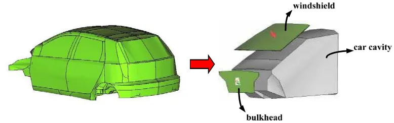
Figure 1.1 shows division of car structure into three subsystems to predict the sound pressure
level in the cabin due to force applied on the bulkhead. The subsystems can be divided into
car cavity, windshield, and bulkhead. The noise in the cabin is expected to directly radiate
from the bulkhead to the windscreen causing the screen to vibrate and eventually radiate
noise into the cabin.
Figure 1.1 Illustration of subsystem division in the SEA model.
Because SEA is based on the statistical behaviour of the responses, therefore several
assumptions apply:
(a) Behaviour of the subsystem is dominated by resonances
A larger number of resonant modes in a frequency band smoothes the response spectra
and the spatial variation in the responses (provided that the damping in the subsystems
is not too large).
(b) Weak coupling between subsystems
This is to allow ’control’ of energy flow among the subsystems. In this case, the damping
in both subsystems should be much larger than the coupling between subsystems. This
means that almost all power dissipates in the excited subsystem and one subsystem does
not affect the other subsystems.
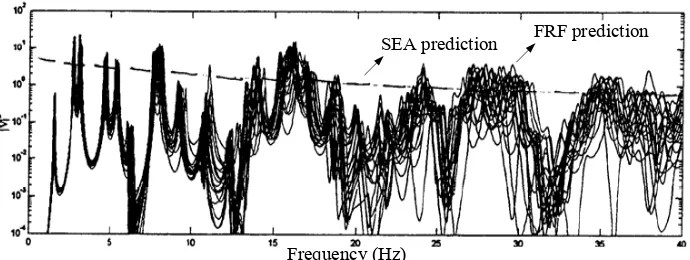
Figure 1.2 shows example of a frequency response function (FRF) compared with the
SEA prediction. At low frequency, the SEA can be seen to have large discrepancy with the
Frequency (Hz)
SEA prediction FRF prediction
Figure 1.2 Comparison between FRF and SEA predictions.
distinct peaks in the graph (in this example below 15 Hz). The FRF can be seen to approach
the SEA prediction at mid to high frequency as the modal density grows rapidly at higher
frequency.
Figure 1.3 shows the typical frequency response of a structural-acoustic system,
indi-cating frequency range of applicability for Finite Element Analysis (FEA), Boundary
Ele-ment Method (BEM) and Statistical Energy Analysis (SEA). The SEA is best to predict the
ensemble average at mid to high frequencies (Kenny, 2002).
9DULDQFH
$YHUDJH
1.2 Past researches on the SEA model development and its application
Statistical Energy Analysis (SEA) was developed in 1960 by Lyon (1967) to predict the
response of launch vehicles to rocket noise and to overcome the limitations of computational
methods. He found that the power flow was proportional to the difference in uncoupled
energies of the resonators and that it always flow from the resonator of higher to lower
resonator energy. A complex structure was breached into subsystems and then stored and
exchanged vibrational energy between these subsystems were analyzed.
The coupling loss factor (CLF) is the most important SEA parameter to be obtained
from the SEA method. It represents how the energy flows from one subsystem to other
sub-systems. Good predictions of CLF is therefore critically important to obtain good estimation
of the noise and vibration in a system. Price and Crocker (1969) formulated the CLF
be-tween room and cavity, assuming that transmission from room to cavity is the same as
trans-mission from room to room. Cushieri and Sun (1994) presented a method for determinating
the dissipation and CLF from SEA model of a fully assembled machinery structure. The
method is based on the experimental measurements of the total loss factors and the energy
ratios between the subsystems of the machine structure when they are fully assembled. Yap
and Woodhouse (1996) investigated the effects of damping on energy sharing in coupled
systems. The approach taken is to compute the forced response patterns of various idealised
systems, and from these the parameters of the SEA model for the systems are calculated.
Mace (1998) predicted the coupling loss factor using SEA theory for systems
consist-ing of rectangular plates. It is found that if the dampconsist-ing is large enough (weak couplconsist-ing)
the response is independent of the shape of the plates and for lighter damping (strong