SPECTRAL REPRESENTATION IN SABANG AND JEPARA COAST

(1)

34 Spectral Representation in Sabang and Jepara Coast

SPECTRAL REPRESENTATION IN SABANG AND JEPARA COAST

R

EPRESENTASI

S

PEKTRUM DI

P

ANTAI

S

ABANG DAN

J

EPARA

Setiyawan

Doctoral Program, Civil Engineering and Enviromental Department, Bandung Institute of Technology Ganesha 10 Bandung 94118 e-mail: [email protected].

ABSTRACT

India ocean in optimation theoretical wave spectrum only wide spectrum and peak frequency equalized but peak energi not yet equalized hence in this research will equalize wide spectrum, peak frequency and peak energi for indonesia ocean that is Sabang coast and Jepara coast. About 12 mounth measured wave spectra from the Sabang Coast and 2 month from the Jepara Coast, were analyzed so as to determine the frequency of occurrence of peaked spectra in sea states of different intensity. This type of spectrum did not occur so often close to coast and in high sea states. A four-parameter theoretical formulation was proposed to represent peaked spectra and was shown to provide an excellent fit to measured spectra. The average values of the spectral parameters describing the two peaks did not show any clear dependence on significant wave height. The mathematical spectrum models are generally based on one or more parameters, e.g., significant wave height, wave period, shape factors, etc. The most common single-parameter spectrum is the Pierson-Moskowitz model based on the significant wave height or wind speed. There are several two-parameter spectra available. Some of these which are commonly used are Bretschneider, ISSC and ITTC. JONSWAP spectrum is a five-parameter spectrum, but usually three or the parameters are held constant. Qualitative as well as quantitative comparisons of the optimation-yielded spectra with target spectra indicated that the developed optimation could model the wave spectral shapes in a better way than commonly used theoretical spectra.

Key words: Sabang Coast; Peaked spectra; JONSWAP spectrum; Significant wave height; Spectral energy

ABSTRAK

Pantai India telah dilakukan optimasi spektrum gelombang teoritis hanya lebar spektrum dan puncak frekuensi yang disamakan tetapi puncak energi tidak disamakan sehingga penelitian ini akan menyamakan lebar spektrum, puncak frekuensi dan puncak energi untuk laut indonesia yaitu pantai Sabang dan Pantai Jepara. Pengukuran 12 bulan spektrum gelombang Pantai Sabang dan 2 bulan Pantai Jepara, yang dianalisis sesuai dengan perhitungan frekuensi kejadian dari puncak spektrum dalam kondisi laut dari intensitas yang berbeda. Tipe spektrum ini tidak terjadi untuk pantai tertutup dan dalam kondisi laut tinggi. Rumus teoritis empat-parameter yang diusulkan untuk merepresentasikan puncak spektrum dan menunjukkan yang cocok dengan spektrum observasi. Nilai rata-rata dari parameter spektrum menggambarkan dua puncak tidak terlihat beberapa tergantung dari tinggi gelombang signifikan. Model spektrum matematika biasanya berdasarkan satu atau lebih parameter, misalnya, tinggi gelombang signifikan, periode gelombang, faktor ketajaman, dan lain-lain. Salah satu spektrum satu parameter adalah model Pierson-Moskowitz berdasarkan tinggi gelombang signifikan atau kecepatan angin. Ada beberapa spektrum dua parameter yang sesuai. Beberapa diantaranya yang digunakan adalah Bretschneider, ISSC dan ITTC. Spektrum JONSWAP adalah spektrum lima parameter, tetapi biasanya tiga parameter dianggap konstan. Seperti halnya perbandingan antara qualitatif lebih baik dari quantitatif dari optimasi spektrum lapangan sebagai target indikasi spektrum bahwa pengembangan spektrum dapat model ketajaman spektrum gelombang lebih baik daripada spektrum teoritis yang digunakan.

Kata kunci: Pantai Sabang; Puncak spektrum; Spektrum JONSWAP; tinggi gelombang signifikan; Spektrum energi

INTRODUCTION

In the 50s, several expressions have been proposed to represent the sea spectra. It seems that a general consensus has been reached later, as to the adequacy of the Pierson-Moskowitz spectrum (Pierson and Moskowitz, 1964) to represent fully developed sea states. This is expressed in the

(2)

Eco Rekayasa/Vol.9/No.1/Maret 2013/Setiyawan/Halaman : 34-41 35

average period since these are the long-term statistics used in ship design. This form has become known as the ISSC spectrum (Soares, 1984).

Developing seas have a more peaked spectrum, as has been demonstrated during the JONSWAP project by Hasselmann et al. (1973). They proposed a spectral form that accounted for the dependence on the wind speed and fetch. Since then, several independent studies have indicated the adequacy of that spectrum to fetch limited situations although suggesting slightly different values of the spectral parameters (Mitsuyasu et al., 1980). The JONSWAP spectrum has also been recommended by the ISSC shape of measured spectra is presented by Haver and Moan (1983). However, both of these formulations represent single peaked spectra while many measured spectra exhibit two peaks. This occurs when there is simultaneously swell and wind sea present or when a refreshing or a changing direction wind creates a developing wave system (Soares, 1984).

Design of marine structures is based on estimates of the maximum wave induced loads expected to occur during a given return period. Wave induced motions and loads are generally determined in the frequency domain. The short term response spectrum is obtained as the product of an input wave spectrum by a transfer function. Design values of loads are then obtained by combining the short-term responses with the long-term variation of the sea state parameters. In this calculation procedure the choice of the wave spectral shape has an important effect on the resulting design loads (Soares, 1984).

Although this is a quite common situation, response calculations are mostly done with single-peaked spectra (Fukuda, 1967: Soding, 1971; motions of marine structures. The proposed spectrum is defined by four parameters, whose typical values are assessed from a data base of 12 mounth measured spectra from Sabang and 2 month from Jepara, a coastal station in the South Java Coast and Jepara Coast.

REPRESENTATION OF THE VARIABILITY OF SPECTRAL SHAPES

The one-dimensional frequency spectrum of waves often forms a prerequisite to trials in structural design, simulation of random waves in a laboratory, as well as study of a variety of coastal processes, like wave refraction and sediment transport. The spectrum of waves can be derived from a specified design value of the significant wave height alone or in combination with that of the average wave period (normally made available to designers by analysis of visual observations, wind–wave relations, or statistical analysis of wave heights) by using empirical relationships, like those of Pierson– Moskowitz (PM), JONSWAP, and Scotts. Many of Dattatri et al.(1977) and Narasimhan and Deo (1979) have shown inadequacy of the most common spectra of PM and JONSWAP to Indian locations (Nameekar, 2006).

The theoretical spectra had been derived on the basis of statistical curve fitting to field observations. In the recent past, soft computing techniques like artificial neural optimation (ANN) have proved to be a better alternative to many statistical schemes, e.g., Karunanithi et al.(1994) and Thirumalaiah and Deo (2000). This is presumably due to the ability of ANN to catch the hazy input–output dependency in a “model-free” and “data-oriented” manner with considerable flexibility and adaptability (Nameekar, 2006).

OBSERVATIONS AND ANALYSIS

(3)

36 Spectral Representation in Sabang and Jepara Coast turn towards its right. Subsequently wind magnitude decreased. During early morning hours the wind had a component oriented towards the sea: this is the land breeze. Its magnitude was much weaker than that of the sea breeze. In fact, minimal wind speed of about 1.5m/s was observed around 600 hours. Before commencement of the sea breeze, the wind speed generally remained less than 2m/s. The onset of sea breeze was marked by an abrupt change in wind direction. The wind was from about 90° before 1000 hrs and after onset of sea breeze the direction changed to about 300°. During 1000–2000 hours the wind direction changed slowly from 300° to about 360°. The coastline in the vicinity of Indonesia is oriented along approximately 340°. Hodographs similar to the one shown have been observed at Goa, India (Simpson 1994).

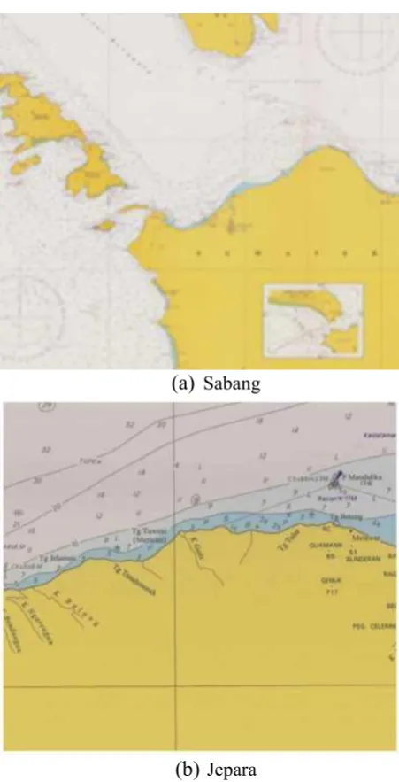
(a)

Sabang

(b)

Jepara

Figure 1. Locations showing the measured wave data used in the study (Bakosurtanal, 2010)

Table 1. Measurement duration, percentage of data with significant wave height more than 2m considered in the present study, water depth and the percentage of spectral energy beyond frequency range of 0.05–0.25 and 0.04–0.35Hz at the location of measurements

Location number 1 2

Water depth at location of measurement (m)

Sabang (20.0)

Jepara (25.0) Measurement duration 12 months 2 months Percentage of data with Hs<2m

considered in the present study 22.19 3.05 Percentage of spectral energy (average

value) beyond frequency range of 0.05– 0.25Hz

58.47 1.94

Percentage of spectral energy (average value) beyond frequency range of 0.04– 0.35Hz

79.17 95.83

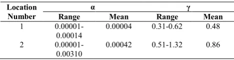
Table 2. The range and average value of wave parameters of the data considered in the study along with water depth at the location of measurement

Wave parameter

Water depth at location of measurement (m) Sabang (20.0) Jepara (25.0) Hs (m) 0.75-3.93 (1.67) 0.16-2.61 (0.96)

T02 (s) 4.8-19.45 (9.49) 4.67-7.14 (5.63)

Tp (s) 16.43-36.97

(23.81)

8.73-14.26 (10.64)

Maximum spectral energy

(m2_/Hz) 0.46-8.36 (2.06) 1.02-5.37 (1.77)

Peakedness parameter (Qp) 0.31-0.62 (0.48) 0.51-1.32 (0.86)

Values inside the bracket indicates average value. Hence, the sea breeze at a height of about 50m above sea level recorded by the anemometer is almost oriented along the coastline. At sea level, the breeze is expected to be at an angle somewhat lower than the angle at the height of the anemometer owing to veering from frictional effects in the atmospheric boundary layer (Neetu, 2005).Various theoretical spectra used for comparison with the measured spectra are given below (Kumar, 2008)

JONSWAP Spectrum

The JONSWAP spectrum was developed by Hasselman, et al. (1973) during a Joint North Sea Wave Project and hence the name. The formula for the JONSWAP spectrum can be written by modifying the P-M formulation as follows

(1)

in which

= peakedness parameter

= shape parameter ( afor ω ≤ ω0, and bfor ω > ω0).

Considering a prevailing wind field with a velocity of Uw and a fetch the average values of these quantities

(4)

The value of a is considered to be the same as in the P-M formula for the fetch independent case. The P-ε and JηζSWAθ spectra are compared. The value of 3.3 yields a mean spectrum for a specified wind speed, Uw, and a given fetch length, X.

However, the value of will vary even for a constant wind speed depending on the duration of the wind and the stage of the growth and the decay of the storm. The values seem to follow a normal probability distribution. Ochi (1978) presented a family of curves for five different values of in the range of 1.75 and 4.85 along with their weighting factors based on the probability density spectrum. He suggested using the family of JONSWAP wave spectra in the design of an offshore structure in a fetch limited area. Thus, for a given significant height and peak period, the response is computed for all five JηζSWAθ spectra for the five values. Then, the desired response amplitude is computed by averaging the responses based on these five spectra and their appropriate weighting factors (Chakrabarti, 1975).

The JONSWAP spectrum is usually considered as a two-parameter spectrum in terms of and ω0,

and α, a and b, are taken as constants with values

prescribed earlier. However, in a design case, usually the significant height and average period of a random wave are specified. Unfortunately, the moments, mn of the JONSWAP spectrum may not be obtained simply in a closed form and the values of and T0 are

calculated numerically by trial and error from Equation 2 using Hs and Ts. A detailed analysis of the

relationships among these four parameters showed that Hs and Ts may be related to T0 and by the

following two polynomial equations:

T0and by the following two polynomial equations:

(2)

And

(3)

From the above equations, for

(4)

which has an error of less than 1% for P-M spectrum (Equation 4) and

(5)

with an error of about 0.1 % (Equation 5).

ISSC Spectrum

The International Ship Structures Congress (1964) suggested slight modification in the form of the Breischneider spectrum,

(8)

Bhattacharyya (1978) discussed this form with the definition of ω= ω0,1. The relationship between the

peak frequency, ω0 and ω for ISSC spectrum is

(Chakrabarti, 1975)

(9)

Goda (1979) derived an approximate explosion for the JONSWAP spectrum in terms of Hs and ω0, as

follows:

(6)

Where

(7)

ζote that for = 1, α* = 0.γ1β which reduces to the P-M spectrum (Equation 7).

Table 3.JONSWAP parameters estimated from the measured wave spectra for different locations

Location Number

α γ

Range Mean Range Mean

1 0.00001-0.00014

0.00004 0.31-0.62 0.48

2 0.00001-0.00310

0.00042 0.51-1.32 0.86

ITTC Spectrum

The International Towing Tank Conference (1966, 1969, 1972) proposed a modification of the P-M spectrum in terms of the significant wave height and zero crossing frequency, ωz. The average zero

crossing frequency is calculated from

(10)

where mn is defined in Equation (10). The ITTC

spectrum has been written as

(11)

Where

(12)

and (13)

in which , the standard deviation

(r.m.s. value) of the water surface elevation. If k = 1, Hsis related to ωs as

(5)

38 Spectral Representation in Sabang and Jepara Coast

Alternativerly, the peak frequency, ω0 from the ITTC

spectrum, Equation (16) is obtained as

(17)

which is the same form as in the P-M spectrum. Since the two spectral forms, Equation (17) and (18) are the same, the characteristic frequency for the ITTC spectrum is ω0 (Mathews (1972)] and the ITTC

spectrum is the same as the modified P-M spectrum. Other forms of ITTC spectrum for different values of k and for different characteristic periods have been discussed by Mathews (Chakrabarti, 1975).

RESULTS OF FIELD DATA ANALYSIS

The analysis in the present study was restricted from the wind-seas. Contribution of the swell waves was insignificant for the period studied here. March– April are the months during which transition from northeast monsoon (November–February) to the much stronger winds of the southwest monsoon occurs. Along the west coast of India the winds due to the latter generally start blowing from the west in May. They strengthen once the monsoon sets in. The period we have analyzed is therefore rather special: the large-scale winds were particularly weak and hence the diurnal cycle due to sea breeze could be identified (Neetu, 2005).

OPTIMATION THE THEORETICAL

FORMULATION TO MEASURED SPECTRA

The theoretical formulation of the double-peaked spectrum has been tested by optimation about half of the 224 measured double-peaked spectra in the Jepara Coast. The criterion governing the choice of the spectra to be tested was a coverage of the various significant wave height groups and a clear distinction between the two peaks. In general, a good

fit was obtained, as can be seen in the selected examples. High wave conditions exhibit mostly a swell dominated spectrum (SR > 1.0). However,

moderate and low sea states have both types of spectra, with SR large and smaller than 1.

The effect of using = γ or = β in optimation a double peaked spectrum can be seen by comparing with the corresponding spectra. The differences are small and result in an improvement and in a degradation of the fit in each of the two cases. This observation of the relative unsensitiveness of the representation to values of justifies the use of an average in all the cases. It also emphasizes the point that = β is a reasonable choice of mean value for the Jepara Coast data. The best fit of individual spectra yields values of , that scatter around the value of β.0.

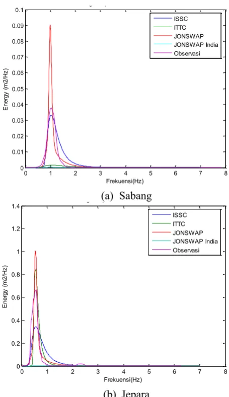
0 1 2 3 4 5 6 7 8

Figure 2. Measured spectra with theoretical spectra

(6)

giving an appearance of two peaks where only one should be considered.

Although using this reduced peakedness of the spectrum, sometimes the theoretical spectrum was still more peaked than the measured one. Two main causes contribute to this fact. Sometimes measured spectra exhibit too much high or low frequency noise, as can be seen in the SN spectra. This contributes to

increase the total energy of the spectrum, as expressed by Hs. As the theoretical model

concentrates the energy near the peak frequencies, they become somewhat overestimated.

The other reason has to do with the width of the spectral bands. While the spectra of Moskowitz et al., Bretschneider et al. and of Snider and Chakrabarti use spectral bands of 0.0055 Hz, Hoffman and Miles use 0.008 Hz and Ewing and Hogben use 0.01 Hz. This means that the sampling interval in the last study is almost twice as large as in the first one. Using a larger spectral band generally underestimates the spectral peaks, which occur between two sampled points. Most of the overpeaked spectra obtained were connected with the studies that used wider spectral This procedure decreased the average wave period by 12% and made the fitted spectrum agree well with the measured one.

It must be stressed that Ewing and Hogben perform this procedure systematically in all the spectra they present. That is, after removing the noise and introducing a calibration factor, they correct the high frequency spectral ordinates to make them follow the shape of the saturated spectrum in the tail. This affects the spectral ordinates for frequencies larger than 0.2 to 0.25 Hz. content, being possible to change their center of area by the inclusion or removal of low energy in the high frequency components.

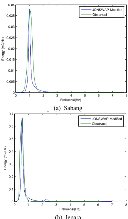
Figure 3. Measured spectra with theoretical spectra and estimated using JONSWAP with modified

parameter

This effect was noticed in several of the low sea states spectra fitted. The data available for sea states under 2 m of significant wave height was mostly translation of the spectrum to lower frequencies.

Table 4. Method of Bretschneider Modification

(7)

40 Spectral Representation in Sabang and Jepara Coast Table 5. Method of Pierson Moskowitz Modification

Modification

Table 6. Method of ISSC Modification

Modification

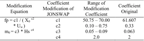
Table 7. Method of JONSWAP Modification

Modification due to the high frequency part of the spectrum. This problem can be solved either by introducing an

The foregoing sections presented development of an optimation in order to estimate the wave surface spectral density function over a wide range of wave

frequencies out of the specified values of the significant wave height and the average zero-cross wave period, which are normally made available to designers by visual observations, wind–wave relations, or statistical analysis of wave heights. The trained optimation when tested for unseen inputs showed that the optimation can be a viable option in order to estimate the shape of wave spectrum. This was evident from the high values of the coefficients of correlation and low values of the mean square as well as mean absolute errors between the optimation-predicted and the target spectral density. The comparison with observed values revealed that the optimation-predicted spectral shapes were more satisfactory than those yielded by the theoretical spectra of Bretschneider, Pierson Moskowitz, ISSC and JONSWAP. While use of the available wave time history could be more beneficial for training, the optimation can also reasonably learn from the theoretical spectra, albeit with reduction in resulting accuracy. The JONSWAP parameters can be estimated using the following expression:

1.12 2.03 1.04 grateful to Dr Sri Legowo, Research Division, for his constructive comments about the initial version of the manuscript. Thanks are also due to Mrs Desyanti for the typing work.

REFERENCES

Bakosurtanal, 2010. Peta Bathimetri Indonesia, Pantai Sabang dan Jepara. 24-26. Jakarta

Chakrabarti, S.K. and Snider, R.H. 1974. Wave statistics for March 1968 Jepara Coast storm. J. geophys. Res. 79, 3449-3456.

C. Guedes Soares, 1984. Representation Of Double-Peaked Sea Wave Spectra. Ocean Engineering, Vol 11, No. 2. pp. 185-207.

Dattatri, J., Jothi Shankar, N., Raman, H., 1977. Comparison of Scott spectra with ocean wave spectra. Journal of Waterway Port Coastal and Ocean Engineering, ASCE 103, 375–378.

Fukuda, J. 1967. Theoretical determination of design wave bending moments. Japan Shipbldg Marine Engng 2 (3), 13-22.

Goodrics, G.S. et al. 1969. Technical decisions and recommendations of the seakeeping committee. 12th Int. Towing Tank Conf., Rome, pp. 821-822.

Haver, S. and Moan, T. 1983. On some uncertainties related to the short term stochastic modeling of ocean

waves. Appl. Ocean Res. 5, 93-108.

Hasselmann, K. et al. 1973. Measurements of wind-wave growth and swell decay during the Joint South Java

(8)

Hogben, N. et al. 1976. Environmental conditions. Report of Committee i. 1, 6th International Ship Structures Congress, Boston.

ISSC, 1979. Report of committee I.1 (Environmental condition). Seventh International Ship Structures Congress, Paris.

Mitsuyasu, H. et al. 1980. Observation of the power spectrum of ocean waves using a cloverleaf buoy. J. phys. Oceanogr. 10, 286-296.

Moan, T., Syvertsen, K. and Haves, S. 1977. Dynamic analysis of gravity platforms subjected to random wave

excitation. Spring Meeting/STAR Symposium, S.N.A.M.E., pp. 119-146.

Narasimhan, S., Deo, M.C., 1979. Spectral analysis of ocean waves a study. In: Proceedings of the Conference

on Civil Engineering in Oceans, vol. 1. ASCE, New York, pp. 877–892.

Nordenstrom, N., Faltinsen, O. and Pedersen, B. 1971. Prediction of wave induced motions and loads for Catamarans. Proc. Offshore Technology Conf., No. OTC 1418, Vol. II, pp. 13-58.

Ochi, M.K. 1978. Wave statistics for the design of ships and ocean structures. Trans. Soc. nay. Archit. mar. Engrs, N.Y. 86, 47-46.

Pierson, W.J. and Moskowitz, L. 1964. A proposed spectral form for fully developed wind seas based on the

similarity theory of S.A. Kitaigorodskii. J. geophys. Res. 69, 5181-5190.

Soares, C. G. 1984. Representation Of Double-Peaked Sea Wave. Ocean Engineering, Vol 11, No. 2. pp. 185-207.

Soding, H. 1971. Calculation of stresses on ships in a seaway. Schiff Hafen 2,3, 752-762.

V. Sanil Kumar, K. Ashok Kumar, 2008. Spectral characteristics of high shallow water waves, Ocean

Engineering 35, pp 900–911.

Warnsinck, W.H. et al. 1964. Environmental conditions. Report of Committee 1, 2nd International Ship