DOI: 10.12928/TELKOMNIKA.v11i3.784 537
The Research of Granular Computing Applied in Image
Mosaic
Xiuping Zhang
School of Computer, Tonghua Normal University, Tonghua city, Jilin Province, China,134002 e-mail: [email protected]
Abstrak
Berdasarkan teknologi mosaik citra yang ada saat ini, makalah ini memperkenalkan komputasi granular dan menghasilkan algoritma baru yang disederhanakan. Citra mosaik dieksekusi dengan algoritma ini pada model korelasi mantap pertama berbasis teori komputasi granular, dan menghasilkan peta tepi dari setiap citra yang membutuhkan mosaik. Metode kalkulasi baru ini digunakan untuk menghitung gradien pada kolom yang berbeda dari peta tepi, untuk mendapatkan koordinat titik fitur dengan gradien maksimum. Semua titik fitur dari dua citra dicocokkan satu sama lain, untuk memperoleh titik kecocokan terbaik. Mekanisme koreksi galat juga diperkenalkan dalam proses pencocokan, yang digunakan untuk menghapus titik fitur dengan kesalahan pencocokan. Perhitungan korelasi dilakukan untuk pencocokan piksel terakuisisi, untuk mendapatkan matriks fitur transformasional dua citra di atas. Berdasarkan matriks tersebut, dua peta citra terpisah dipetakan ke dalam bidang yang sama. Metode transisi mosaik lambat ini diterapkan dalam aspek penambahan dan penghapusan tumpang tindih citra, sehingga citra tidak memiliki batas menonjol setelah mosaik. Seluruh proses mosaik citra menunjukkan bahwa algoritma komputasi granular yang diusulkan lebih unggul dibandingkan dengan mosaik tradisional baik dari sisi jumlah citra terproses maupun jumlah pengolahan. Selain itu, citra mosaik yang dihasilkan juga memiliki kualitas yang lebih tinggi.
Kata kunci: butir informasi, komputasi granular, mosaik citra, titik fitur
Abstract
Based on the existing image mosaic technology, this paper introduces the granular computing and obtains a simplified new algorithm. The image mosaic executed by this algorithm at first establishes correlation model on the basis of granular computing theory, and obtains edge map of each image needing mosaic. The new calculation method is used to calculate gradient of in different columns of edge map, to obtain the feature point coordinates with the maximum gradient; meanwhile, all feature points of two images are matched with each other, to acquire the best matching point. In addition, the error-correcting mechanism is introduced in the matching process, which is used to delete feature points with matching error. The correlation calculation is carried out for the matching pixels acquired by the above processing, to get the feature transformational matrix of the two images. According to the matrix, two separated image maps map into the same plane. The slow transitional mosaic method is applied in the aspect of image addition plus overlap removal, so that images have no bulgy boundary after mosaics. The whole image mosaic process shows that the given granular computing algorithm is superior to the traditional one both in the number of processed images and the number of processing, and the mosaic image gained has high quality.
Keywords: feature points, granular computing, image mosaic, information granule
1. Introduction
domain, conducting Fourier change for images, to acquire related transformation parameters and overlap region. This method is often limited by the nature of image, which is only applicable to the 2n×2n image having linear gray value. The third one is a computation method based on image features, in which each pixel point has its unique symbol characteristics, for example, feature points. Through the pixel processing, the symbol characteristics can be acquired, which are matched with each other, and the area with similar altitude feature belongs to the matching area. This method has significant pixel features and prominent advantages in the process of contrast image mosaic, which have been widely promoted.
The definition of granular computing [1] is put forward by T.Yin in 1997, and its main content is to decompose the research object with complex structural into multiple different levels of elements. It conducts a good analysis of complex object under different granularities. This method can more directly observe the essence of the object, so as to further study the object and reduce a lot of unnecessary researches. With many years of development, the technology has been widely applied in many fields, such as image processing, knowledge discovery, D-S theory and so on.
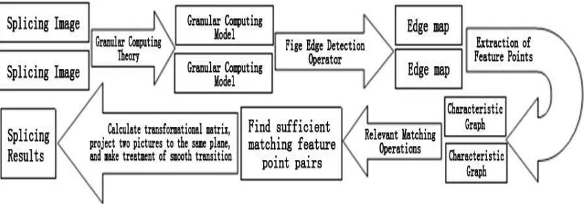
Image mosaic is a very important image processing. This paper fully applies the granular computing method to the third splicing computation method based on the above, thus construct a new image mosaic computation method. The specific process for new computation method shows in the Figure 1.
Figure 1.Image Splicing Process Based on Granular Computing Theory
2. Granula Computing Principles
Due to the limited ability to solve current problems, according to inherent characteristics, all the data parameters of complex problems are often classified as different small data block, which are called information granule in computer language, so as to solve the problem containing in many data information. From this concept, as a mathematical set, information granule contains many elements with similar characteristics. However, granular computing is aimed at scientific processing for each refining information granule. The essence of technology is to decompose the complex object difficult to be studied into different levels of information granule for related computation,
Conduct statistical analysis of all data of information granule acquired, to achieve the optimal scheme.
granules. And conduct hierarchical classification according to the size of information granule, and then carry out the data processing for each layer of information granule.
After the problem is disintegrated, the granular computing theory can greatly reduce the complexity of problem solving, which belongs to a technology with wide applicability. The following text will give the definition of key process related to the theory [3]:
Definition 1-1: based on the domain granularity decomposition and coverage, assuming that there is a mutual relationship of domain U and each element in the U,
: ( ), i i
R UP U U
G, in the reasoning process,{ }
G
i irepresents an information granule,and P U( ) represents U’s power set. The domain relation R has more categories, which can be
similarity relation, equivalence relation, fuzzy relation, etc. When
i j
,
,i j G Gi j, and{ }
G
i i means domain granularity partition; when
i
,
j
,i j GiGj , and then{ }
G
i i is called “Domain Granularity Coverage”.Definition 1-2 refers to mathematical set of information granule: assuming that there is a domain U, and this domain granularity is divided as
i i
U G, and the size of granule G is called ( ) ( )
G
d G Card G G
dx. The fuzzyinformation granule is expressed as the equation: G ={x
G x( ) 0, x U}.The specific process of granular computation includes the following steps: (1)according to the object of study, give the expected goal of domain U; (2) based on the expected goal of domain, define level number of information granule design, and establish related structure model; (3) according to the characteristics of information granule division, and adopt the scientific and reasonable method for calculation; (4) repeat inflammation, and get the best solution.
3. Application of Granular Computing Theory to Detection of Image edge
3.1. Information Granule Structure Classification of Image Plane and Image Fuzzy Information: Granule Digital Representation
The granular computing theory is applied to the image processing process. The specific image is frequently regarded as an information system, and the gamma gray-scale is adjusted to [0, 1]. In the image domain, the relationship R involved is fuzzy relation
R
F X Y
(
)
, which represents the M * N gray-scale map [4]. Two coordinate axes x and y of two-dimensional image set up the corresponding fuzzy sets P and Q, P = {P1, P2,... , PI}, Q = {the 25th, Q2,... , QJ}, in the fuzzy set, element Pi and Qj belong to information granule in different directions. Through t modular arithmetic of information granule in two different directions, we can acquireinformation granule in two-dimensional system Tij:
T x y
ij( , ) (
P Q x y
i j)( , )
P x tQ y
I( )
J( )
, alsoknown as Cartesian Information Granule, thus the image information partition is completed. In the division of different information granule, there are multiple image pixels, so no need to discuss image pixels.
Definition 3-1 two fuzzy sets’ generalized inner product and generalized outer product:
assumed thatA B, F X( Y), and sup( ( , ) ( , ))
, y x tB y x A B A y x
and inf( (, ) ( , ))
, AxysBxy
B A
y x
are
generalized inner product and generalized outer product of two fuzzy sets, A and B respectively. The definitions of R and Tij are stated as before, supposed that gijR T ijR(P Qi j),
( , )i j I J , and then the fuzzy information granule can be expressed as mathematic expression G=[gij]I×J. The information granule determinacy and the size of fuzzy relation are inversely proportional. The more specific information granule has structure, the more it objectively represents the original pixel information.
3.2. Using Fuzzy Information Granule Edge Operator for Image Detection
( , ) ( )( , ) ( ) ( )
ij i j I J
T x y P Q x y P x tQ y , and the complementary set of two-dimensional information
granule set is expressed as c( , ) 1 ( , )
T x y T x y . Then the image gray-scale can be expressed by T R and c
T R, so as to acquire the adaptability calculation formula of image information
granule, L P Q R( ; ; )T R T cR . Through the above formula, we can obtain the adaptability of Cartesian information granule T of the image to the whole image. The L(X;Y;R) size and adaptive size are inversely proportional, and the best adaptability corresponds to the minimum L(X;Y;R)
The adaptability of image information granule is related to its structure and its pixel gray-scale contained. Assuming that the former is constant, the adaptability of information granule is only related to its pixel gray-scale contained, so that the edge of image area can be determined well. Granular computing application creates a new-type image edge determination method, called Edge Operator of Fuzzy Information Granule (Fige Operator).
Assuming that image contains two domains
X
{ , ,..., }
x x
1 2x
andY{ , ,..., }y y1 2 y , fuzzy setsareP F X ( ) and Q F Y ( ); through the fuzzy sets P and Q, T and Tc, we can acquire two-dimensional information granule of the image, representing fuzzy matrix β×β, of which the determinants include coordinate axis information granule, t modular operator and matrix size β of two coordinate axes.
The 3×3 edge operator is expressed as: assuming that fuzzy sets, P and Q, meet
2
( m) exp{ ( 2) }
P x
m andQ y( n)exp{
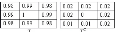
(n2) }2 , among them, 0.01 and m n, 1, 2,3. Adopt t module (p=1) defined by Yager and its dual module s [5]:1 1 (2 ) 0 ( 1)
xty x y x y andxsy 1 (x y)generate two convolution kernels, as follows:
T TC
The process in which Fige operator determines image edge is as follows:
Assuming that both tij and tcij are included in the edge operator convolution kernels, T and Tc, and rij represent as gray values of different two-dimensional information granule. Through the logic operation of convolution kernels T and Tc, the monitoring point expands from the center information granule of the image to the edge, covering all the pixels of the image: (1).
calculate
,
sup(ij ij)
i j
T R t tr and
,
inf ( )
c c
ij ij i j
T R t sr ; (2) outputT R T cR
, representing the fitness
of the information granule.
In the process of edge detection of Fige operator, some columns of fitness are acquired, which directly reflect gray value of each information granule, so as to determine the possibility that the information granule belongs to image edge. The parameter σ designed in the fuzzy matrix belongs to a dynamic parameter, which can be adjusted according to the specific situation, and its common value is 0.02. Generally speaking, the dereferencing can acquire effectively image edge. Assuming that the researchers place extra emphasis on main edge or small edge, the dereferencing of parameter σ will be adjusted, and Fige operator detection is conducted again.
3.3. Experimental Comparison of Fige operator and Traditional Edge Detection Operator The traditional image edge detection operator regards Prewitt and Sobel as representative. Compared to the above two kinds of edge detection, Fige operator can greatly reduce the complexity of calculation, and efficiently deal with complex problems, and the computation for design attribute is just simple addition, subtraction and comparison operations. Three kinds of detailed comparison between operators are shown in the Table 1, from which, it can be seen that the Fige operator only has more times in size comparison operation, which is equal to addition operation from the angle of calculation difficulty. It means that the operator runs several times of addition operation in the calculation; however, comprehensively speaking, it is a simple efficient edge detection method.
Figure 2. Influence of Fige Operator Parameter Selection on the Result
Table 1 A Pixel Computation of Three Kinds of Different Operators
Operator Prewitt Sobel Fige
Addition or Subtraction 10 10 4
Big or Small Dereferencing 1 1 7
Shifting 0 2 0
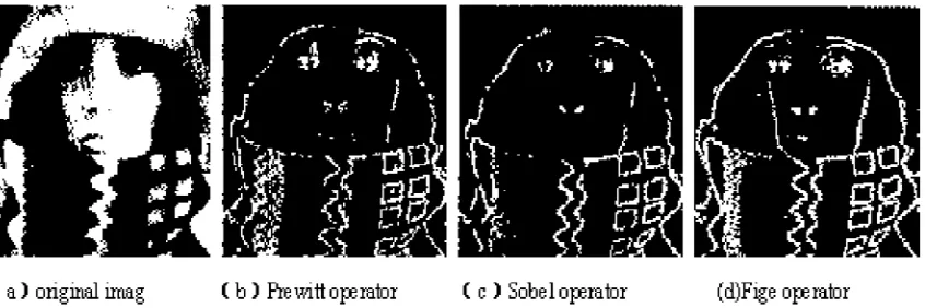
Comparing edge detection results: in the comparative test, the test object is 256x256 images, and the detection methods aim at three kinds of different detection operator, and the Figure 3 describes image edge acquired in three different detection methods in detail. The comparative analysis shows us that the image edge obtained by the traditional operator Prewitt and Sobel is unsatisfactory, its edge information is fuzzy, and there are many breakpoints; but Fige operator can obtain clear edges without breakpoint, and its detection effect is obviously superior to the traditional operator.
4. Image Feature Points’ Extraction and Matching 4.1. Acquisition of Feature Points
Set the width of two plane images, which need to be splicing, as W1 and W2 respectively, the height as H1 and H2 respectively, find the maximum gradient point in all the edge points, which are covered by multiple edge lines in each edge of two images obtained in the Fige operator method, mark and write down its ordinate. If a column corresponding to image edge has no edge point, you only need to contrast the gradient values of all points in this column, and take the maximum. If the point (i, j) is located in the image, the equation of gradient
value is
Magi j
(, ) {[( ( 1, ) ( 1, ))/2] [( (, 1) (, 1))/2]}
I i
j I i
j
2
I i j
I i j
2 1/2, in which, I (i, j) represents the gray value of arbitrary point (i, j). The above two images include W1 and W2 respectively, so as to obtain ordinate sets Mag1 and Mag2 of points, corresponding to the maximum gradient value in each column of image, two sets of element amount are W1 and W2 respectively, which represent the position of the maximum gradient feature point owned by two images. In the image, relevant standards acquired of the maximum gradient point corresponding to each column are as follows: supposing that a column in the image has two or many maximum gradient feature points, when selecting, the point closest to horizontal centerline is generally preferred; assuming that two maximum gradient points not only have equal gradient value, but are same as the closeness degree of horizontal centerline, then the point having large ordinate is preferred.Take marks of all the maximum gradient points of two images obtained in the picture, to obtain their own characteristic graphs F1 and F2 correspondingly.
4.2. Extraction of Matching Feature Points between Characteristic Graphs
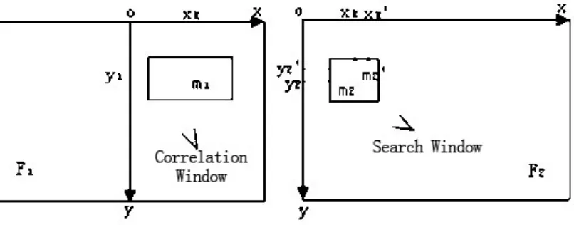
Project characteristic graphs of two images acquired to the same plane. There is about 1/3 to 1/2 superposition area in two splicing images; therefore, when matching the characteristic graph, Y axis is determined by the perpendicular bisector of characteristic graph F1. Thus, when matching, it can reduce the workload, only matching F1 right area and F2 left area, and Figure 4 describes the matching process of feature point in detail.
Figure 4. Diagram for Search Matching Feature Points of Two Images
In order to quickly calculate the matching area of two characteristic graphs, this paper applies the new calculation method, and the details are as follows:
- Through the matching contraction of characteristic graph F2 from right to left, the matching feature point, m2 '(xk', y2 '), of m1 is obtained.
Two feature points matching mechanism: at first introduce the parameter m2' of two
feature points m1 and m2', defined as:
1 2 1 2 1 2 ( , ') ( , ') ( ), ( ') Cov m m Score m m
m m
, among them,
1 2
(
,
')
Cov m m
represents the covariance of points m1 and m2' in its correlation window, andthe expression is:
1 1 1 2 2 2
1 2
[ ( , ) ( )][ ( ' , ' ) ( ')] ( , ')
2 1 (2 1)
n m
k k
i n j m
I x i y j E m I x i y j E m Cov m m
n m
(1) 1(
m
)
represents standard deviation of characteristic graph in the search area at the center of point m1 and with the scope of (2n+1)(2m+1), the detailed equation is:2
1 1 1 1
( ) [ ( , ) ( )]
n m k i n j m
m I x i y j E m
. (2)From the correlation equation, it is known that the correlation value Score of two feature points is located in the interval [-1,1], the matching degree of two feature points m1 and m2' is proportional to Score, only when the Score value is more than a threshold value, we can think two points are matching. In the general condition, the Score threshold value is 0.95, only when the Score value between m1 and m2' is more than 0.95, m2' can serve as the candidate matching point of m1.
- Assuming that a feature point has multiple candidate matching points, then the maximum score point is selected as its real matching point. If the optimal matching point cannot be found and determined, it is required to conduct the match computation again.
- Repeat the first three steps, after have probably about 15 feature matching points, cut off the matching.
4.3. Elimination of Mismatching Point
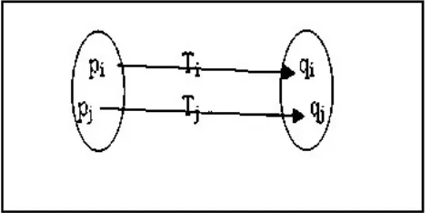
In order to find the mismatching in the matching feature points, it is required to consider eliminating the mismatching feature points. Elimination of mismatching feature points are based on the hypothesis: the rotation and scaling motion of two images are relatively smaller than the translational motion, so the difference should be small of two vectors connecting two adjacent matching points, as shown in the Figure 5.
Figure 5. Eliminating the mismatching feature points
The elimination of mismatching point is based on the following premise: the image translational motion is more frequent than rotation and scaling motion, therefore, the vectors of two matching points are very close, with small difference. The Figure 5 has its logo. Supposing that the
vectors of two matching point are Ti qi pi
and
T
j
q
jp
j
, which are very close, at this time,
compare Ti
with its expected value of adjacent feature point vector, and understand their differences. If the difference is small, it shows that points P and q are correct matching points; if the difference is large, then it is required to eliminate it, in this way, to ensure the accuracy of matching process.
5. Transformation Parameters Solving between Images
Given that two images’ multiple matching feature points, you can get transformation parameters between two graphs, so that two graphs can be projected to the same coordinate system, for the next image splicing.
The mechanism of computing image transformation parameters: in general, there is three-dimensional mapping relationship between two images, in essence, it is three-dimensional mapping between-two planes. Assuming that it is required to take a point PS on the projecting plane, the factor point Pd refers to a point to be projected on the plane, and the transformation parameter is expressed by Msd of the point located in two planes, then there are the following relations:
( ',
',
)
( ', ', )
1
d s sd
a d g
P
P M
x
y w
u v q
b e h
c f
(3)
Transformational matrix Msd has eight degrees of freedom (usually, i=1), in theory, at least 4 pairs of feature point are required to estimate the Msd. Select four optimal matching feature points( , )u vk k ( ,x yk k), and write down 8 equations of unknown number is a-h:
In theory, transformational matrix is the parameter with 8 degrees of freedom, from this point of view, feature points of 4 or above can compute Msd. Next, we select 4 pairs of the best matching points of two images ( , )u vk k ( ,x yk k) to calculate eight different parameters, and the equation is as follows:
1
k k
k k k k k k k k
k k
du
ey
f
y
du
ey
f u x g v x h y
gu
hv
(4)and
k
(
1
,
2
,
3
)
.Through the above equation, we can get a-h eight parameters, so as to estimate the transformational parameter Msd between two images.
6. Smooth Transitions between Images
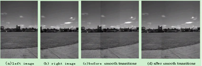
In general, two images used for splicing have different sources, different shooting angles and shooting time, so there is obvious difference in the brightness. If only two images, which are projected to the same plane, are overlapped, the superposition between images will have obvious visual conflict limits. For the seamless connection between images, we often need to make smoothing treatment of superposition, thus the whole picture has a good sense of reality.
two images, g i j( , )dg i j1( , ) (1 d g i j) 2( , ). In the Eq., parameter d is gradient coefficient, and its
size is from 1 to 0. In the process of gradual change of parameters, two images’ gray levels deserve good buffering, so as to avoid the abrupt boundary line. This method is widely applied in the smooth transition image of splicing process, and the splicing image obtained has good effect, but it is often affected by the difference by the resolution of two splicing images. Aiming at this problem, BurtPJ gives the strategy of multi-resolution image mosaic transition [6], and the image with great difference of resolution can also complete seamless splicing.
7. Experimental Results
In this paper, the computer chip used for image splicing is CPU Centrino and its memory size is 512 MB. The splicing process is completed in software visual C++6.0. The Figure 6 shows us the complete image after splicing vividly.
Figure 6.Experimental Results
8. Conclusions
An important research direction for the current image splicing technology is to simplify the related calculation and computational efficiency when completing high-quality image mosaic. The new algorithm based on granular computing has the following advantages: the granular computing theory is used for image processing, to greatly expand the scope and complexity of image processing. The Fige operator established on the basis of this theory, whether in the calculation amount or in the detection efficiency, is obviously superior to the traditional operator. The feature point extraction method required by image mosaic mainly depends on the maximum gradient value of each column of the image, to reduce the complexity of traditional image feature extraction method greatly, having stronger operability. In this paper, based on large superposition area between two images, set ordinate as the perpendicular bisector on the left of images, and only search the general area in two images. Compared to the traditional feature point matching method, it greatly reduces the computation amount and speeds up the matching speed. Eliminate the mismatching for matching feature points found, furthermore, ensure that the matching feature found is the best, and the accuracy of algorithm is improved. To sum up, in the paper, the new algorithm, which is proposed on the basis of granular computing theory, is obviously superior to the traditional algorithm, and can obtain the high-quality overall image, so it should be promoted vigorously.
References
[1] T.Y.Lin. From Rough Sets and Neighborhood Systems to Information Granulation and Computing in Words, European Congress on Intelligent Techniques and Soft Computing, 1997:1602-1606.
[2] Lin T Y. Granular computing: Examples, intuitions and modeling// The 2005 IEEE International conference on Granular Computing, Beijing,China,2005:40-44.
[3] Lin Y, Liu Q. Formalization for granular computing based on logical formulas. Journal of Nanchang Institute of Thechnology, 2006 ,25(2):60-65.
[4] K Hirota, W Pedrycz. Fuzzy relational compression [J]. IEEE Trans. Syst. Man. Cybern. pt. B.June 1999,29(3):407-415.
[5] M Mizumoto.Pictorial representations of fuzzy cnnectines, Part I: Cases of t-norms,l-conorms and averaging operators[J]. Fuzzy Sets Syst.1989.31(2):217-242.