Abstract —Bilinear time-frequency distributions (TFDs) are powerful techniques that offer good time and frequency resolution of time-frequency representation (TFR). It is very appropriate to analyze power quality signals which consist of non-stationary and multi-frequency components. However, the TFDs suffer from interference because of cross-terms. This paper presents the analysis of power quality signals using bilinear TFDs. The chosen TFDs are smooth-windowed Wigner-Ville distribution (SWWVD), Choi-Williams distribution (CWD), distribution (BD) and modified B-distribution (MBD). The power quality signals focused are swell, sag, interruption, harmonic, interharmonic and transient based on IEEE Std. 1159-2009. To identify and verify the TFDs that operated at optimal kernel parameters, a set of performance measures are defined and used to compare the TFRs. The performance measures are main-lobe width (MLW), peak-to-side lobe ratio (PSLR), signal-to-cross-terms ratio (SCR) and absolute percentage error (APE). The result shows that SWWVD is the best bilinear TFD and appropriate for power quality signal analysis.
Index Terms—bilinear time frequency distribution, optimal
kernel, power quality, time frequency analysis
I. INTRODUCTION
Nowadays, power quality has become important because of the usage of electrical equipment in our daily lives. It has become an issue because the presence of the power quality signal can generates higher losses and cause low reliability of the whole systems. Moreover in industrial plants, the effect comes to the reduction of lifetime of the load and the ineffective performance of protection devices. For that reasons, an automated monitoring system is required to provide adequate coverage of the entire system, rectify the causes of these disturbances, resolve existing problems and predict future problems [1].
Manuscript received Dec 10, 2011; revised Dec 30, 2011. This work was supported by Universiti Teknikal Malaysia Melaka (UTeM) .
A. R. Abdullah is with the Electrical Engineering Department, Universiti Teknikal Malaysia Melaka, 76100, Durian Tunggal,Melaka Malaysia, (e-mail: [email protected]).
A. Z. Sha’ameri is with the Electrical Engineering Department, Universiti Teknologi Malaysia, 81310, Skudai,Johor, Malaysia, (e-mail: [email protected]).
N. A. Mohd Said is with the Electrical Engineering Department, Universiti Teknikal Malaysia Melaka, 76100, Durian Tunggal,Melaka Malaysia, (e-mail: [email protected]).
N. Mohd Saad is with the Electronics & Computer Engineering Department, Universiti Teknikal Malaysia Melaka, 76100, Durian Tunggal,Melaka Malaysia, (e-mail: [email protected]).
A. Jidin is with the Electrical Engineering Department, Universiti Teknikal Malaysia Melaka, 76100, Durian Tunggal,Melaka Malaysia, (e-mail: [email protected]).
In current research trend, short time Fourier transform (STFT) [2] is a popular technique for power quality signal analysis. The technique presents the signal jointly in time-frequency representation (TFR) which provides temporal and spectral information. However, it has limitation of a fixed window width that results a compromise between time and frequency resolution. The greater temporal resolution required, the worse frequency resolution will be and vice versa. To overcome the limitation of the fixed resolution of STFT, wavelet transform (WT) was proposed by various researchers [3]. In addition, WT also exhibits some disadvantages such as its computation burden, sensitivity to noise level and the dependency of its accuracy on the chosen basis wavelet [4, 5].
Bilinear time-frequency distributions (TFDs) [6] have been intensively used to characterize and analyze non-stationary signals. The bilinear TFDs offer a good time and frequency resolution and are successfully applied to various real-life problems such as radar, sonar, seismic data analysis, biomedical engineering and automatic emission [7]. However, the TFDs suffer from the presence of cross-terms interferences because of its bilinear structure. This inhibits interpretation of its TFR, especially when signal has multiple frequency components [8]. Some members of the bilinear TFDs are Wigner-Ville distribution (WVD), windowed Wigner-Ville distribution (WWVD), smooth-windowed Wigner-Ville distribution (SWWVD), Choi-Williams distribution (CWD), B-distribution (BD), modified B-distribution (MBD) and Born-Jordan distribution (BJD). An analysis of the auto-terms presentation using the reduced interference distributions (RID) has been discussed [9]. A procedure of designing a kernel that will produce the desired auto-term shape and an optimal kernel with respect to the auto-term quality and cross-term were demonstrated.
In this paper, the SWWVD, CWD, BD and MBD which are the popular bilinear TFDs are chosen to analyze power quality signal. The power quality signals are swell, sag, interruption, harmonic, interharmonic and transient. A set of performance measures to identify the optimal kernels of the TFDs by comparing their TFRs in terms of main-lobe width (MLW), peak-to-side lobe ratio (PSLR), absolute percentage error (APE) and signal-to-cross-terms ratio (SCR). APE is the first consideration because of its ability to quantify the accuracy of signal characteristics that are calculated from the TFR, and then the SCR, MLW and lastly PSLR. From the comparison results, the best bilinear TFD is chosen for power quality signal analysis.
II. SIGNAL MODEL
This paper divides the signals into three categories: voltage variation, waveform distortion and transient signal. Swell, sag and interruption are under voltage variation, harmonic and interharmonic are for waveform distortion and
Bilinear Time-Frequency Analysis Techniques
for Power Quality Signals
transient is for transient signal. The signal models of the categories are formed as a complex exponential signal based on IEEE Std. 1159-2009 [10] and can be defined as
waveform distortion and ztrans(t) represents transient signal. k
is the signal component sequence, Ak is the signal
component amplitude, f1 and f2 are the signal frequency, t is
the time while (t) is a box function of the signal. In this analysis, f1, t0 and t3 are set at 50 Hz, 0 ms and 200 ms,
respectively, and other parameters are defined as below: 1. Swell: A1= A3 = 1, A2 = 1.2, t1= 100 ms, t2= 140 ms
III. BILINEAR TIME-FREQUENCY DISTRIBUTIONS Bilinear TFDs analysis is motivated by the weakness of linear TFDs. Generally, the bilinear TFDs can be formulated as time-convolution of the signals. The bilinear product can be defined as
A. Smooth-Windowed Wigner-Ville Distribution
The SWWVD has a separable kernel [11] which is separated in time and lag components. This technique has the advantages of reducing the effects of interferences or cross-terms and at the same time having a high time and frequency resolution. General expression of the separable kernel is written as
) lag window function. In this paper, raised-cosine pulse is used as the TS function while Hamming window is as the lag-window [12] and are, respectively, defined as
The optimal setting of the separable kernel is different for all types of signal. It has been discussed specifically in [9].
B. Choi-Williams Distribution
The CWD function adopts exponential kernel to reduce interference in TFDs [11] and can be defined as
2
where σ is a real parameter that can control the resolution and the cross-terms reduction. This kernel gives good performance in reducing cross-terms while keeping high resolution with a compromise between these two requirements.
C. B-Distribution
The BD uses positive real parameter that controls the degree of smoothing where the value is between zero and unity [11]. The positive real parameter, β, is defined in time-lag plane where it acts like a low-pass filter in the Doppler domain. Its kernel distribution is defined as
t t
G(,)cosh2 (11)
D. Modified B-Distribution
The MBD was proposed to correct the drawback of the BD which the modification is made in terms of lag-independent kernel [11]. As stated in equation (12), the different can be seen in terms of its denominator
IV. PERFORMANCE COMPARISON
60 80 100 120 140 160 180 -1
0 1
Power Quality Signal
Time (msec)
A
m
p
li
tud
e (
pu)
and resolution of TFRs [12]. In general, an optimal kernel of TFD should have low MLW and APE while high PSLR and SCR.
PSLR is a power ratio between peak and highest side-lobe while MLW is a width at 3dB below the peak of power spectrum [12] as shown in Fig 1. Low MLW indicates good frequency resolution and it gives the ability to resolve closely-spaced sinusoids. PSLR should be as high as possible to resolve signal of various magnitudes.
Fig. 1 Performance measures used in the analysis.
Fig. 1 Performance measures used in the analysis.
Moreover, the SCR is a ratio of signal to cross-terms power in dB. High SCR indicates high cross-terms suppression in the TFR and is defined as
power terms cross
power signal log
10 SCR
(13)
Besides that, APE is also used to present the accuracy of the measurement. The measurement details are discussed in [13] and can be expressed as
% 100
APE
i m i
x x x
(14)
where xi is actual value and xm is measured value.
V. RESULTS
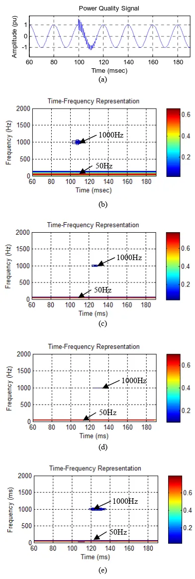
The example of the transient signal and its TFR using SWWVD, CWD, BD and MBD at their optimal kernel is shown in Fig. 2. The line graphs show the signal in time domain while the contour plot demonstrates its TFR. The highest power is represented in red colour while the lowest is in blue colour. The TFR shows that, the transient signal has fundamental frequency along the time axis and a momentary power increase at transient frequency which is at 1000 Hz. However, the duration of the momentary power is different for each plot. SWWVD presents the shortest duration (14 ms) and MBD is the longest (22 ms) while BD (18 ms) is longer than CWD (16 ms). Besides that, the TFR shows some delays compared to input signal because the convolution process between kernel and signal in the TFDs shifted the TFRs in the time domain.
(a)
(b)
(c)
(d)
(e)
Fig. 2 a) Transient signal and its TFR using b) SWWVD at Tg=10 ms and
Tsm=0 ms, c) CWD at = 1.0, d) BD at = 0.05 and e) MBD at = 1.0. 50Hz
1000Hz
50Hz 1000Hz
50Hz 1000Hz
50Hz 1000Hz
0 500 1000 1500 2000
-100 -80 -60 -40 -20 0 20
frequency (Hz)
Po
w
e
r i
n
d
B
-3dB
MLW
PSLR
P
ow
er
in
d
B
81 82 83 84 85 86 87 88 89
0 5 10 15 20 25 30
10 15 20 30 40
MLW APE SCR PSLR
12 12.5 13 13.5 14 14.5
0 20 40 60 80 100 120 140 160 180
0 1.578 6.67 7.5 10
MLW APE PSLR SCR
A. Performance Comparison of Smooth-Windowed Wigner-Ville Distribution
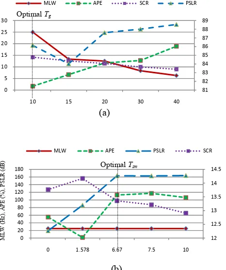
The optimal kernel parameters for the transient signal are at Tg = 10 ms and Tsm = 1.578 ms. To identify the
performance response corresponding to the kernel parameters, the performance measures of the TFR with various kernel parameters are plotted in Fig. 3. The optimal kernel parameters chosen should be low MLW and APE but high PSLR and SCR. As shown in Fig. 3 (a), at optimal value of Tsm and higher Tg, SCR is lower because of the
reduction of the cross-terms suppression. However, it results MLW smaller that indicates higher frequency resolution of the TFR. In addition, higher Tg also increases the APE that
presents lower accuracy of the TFR. As Tg is set at optimal
value while Tsm is higher as shown in Fig. 3 (b), it gives
smaller SCR and constant value of MLW. Besides that, the APE is also higher because higher Tsm reduces the time
resolution of the TFR. Thus, there is a compromise between cross-terms suppression and time resolution to obtain optimal TFR.
The optimal kernel parameters for voltage variation signal are at Tg = 10 ms and Tsm = 0 ms. For this signal, the
use of the TS function does not introduce any improvement in the cross-terms suppression because all cross-terms have no Doppler frequency. For waveform distortion signal, the optimal kernel parameters for harmonic signal are at Tg = 20
ms and Tsm = 7.5 ms while for interharmonic signal are at Tg
= 20 ms and Tsm = 6.67 ms. All cross-terms of these signals
have Doppler frequency and can be removed by using the TS function at optimal Tsm. Higher Tg does not improve the
cross-terms suppression but it is still used to set the frequency resolution of the TFR that can differentiate harmonic and interharmonic frequency component.
(a)
(b)
Fig. 3 MLW, APE, PSLR and SCR of TFR at (a) optimal Tsm with various
Tg and (b) optimal Tg with various Tsm for transient signal.
B. Performance Comparison of Choi-Williams Distribution
The optimal kernel parameters of the CWD for voltage variation, waveform distortion and transient signals are at = 0.05, 0.01 and 1.0, respectively. As example, performance of sag signal using the CWD at various is shown graphically in Fig. 4. The graph illustrates that, when is set higher than its optimal kernel, the MLW and SCR are smaller. Higher increases frequency resolution of the TFR but it reduces cross-terms suppression. As a result, the APE is higher. As is set smaller, the SCR is higher because smaller removes more cross-terms. However, the frequency and time resolution get worse and resulting in higher MLW and APE. Thus, should be chosen based on the signal characteristics and a compromise between time and frequency resolution and cross-terms suppression is required to obtain optimal TFR.
Fig. 4 CWD with various for sag signal
C. Performance Comparison of B-Distribution
For the BD, the optimal kernel for voltage variation signal is at β = 0.001 while waveform distortion and transient signals are at β = 0.05. As instance, Fig. 5 shows the example of the performance of the BD for harmonic signal. The graph shows that, as β is set other than the optimal value, the MLW is similar and the SCR is smaller. This indicates that β does not change the frequency resolution and reduce the cross-terms suppression in the TFR. As a result, the APE is higher.
Fig 5. BD with various βfor harmonic signal
D. Performance Comparison of Modified B-Distribution
Fig. 6 shows the performance of swell signal using various and its optimal value is identified at = 0.05. Since the performance response of the kernel parameter is similar to BD, same discussion can be made for MBD. However, BD gives better accuracy of the TFR which contributes in higher APE. For swell and sag signals, their optimal kernel parameters are at = 0.05, while Optimal Tsm
M
L
W
(H
z)
, A
P
E
(%), P
S
L
R
(dB
)
S
CR (dB)
0 10 20 30 40 50 60 70 80 90
0 2 4 6 8 10 12 14 16
0.001 0.005 0.01 0.05 0.1 0.5 1
MLW APE SCR PSLR
M
L
W
(H
z)
, A
P
E
(%), S
C
R
(dB
)
P
S
L
R (dB)
Optimal
0 10 20 30 40 50 60
0 5 10 15 20 25
0.001 0.005 0.01 0.05 0.1 0.5 1
MLW APE SCR PSLR
M
L
W
(H
z)
, A
P
E
(%), S
C
R
(dB
)
P
S
L
R (
d
B)
interruption, harmonic, interharmonic and transient signals are at = 1.0.
Fig. 6 MBD with various for swell signal
E. The Optimal Performance of the Bilinear
Time-Frequency Distributions
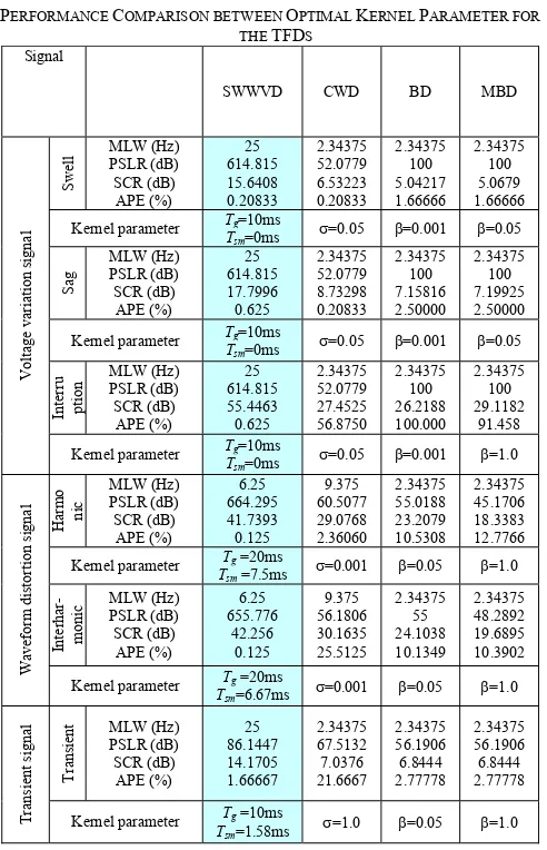
The performance of SWWVD, CWD, BD and MBD at optimal kernel are shown in Table I. The results show that SWWVD is the best distribution for power quality signal analysis. It has good APE, SCR and PSLR but poor for MLW. However, for CWD, BD and MBD the analysis shows that they present good MLW but poor in terms of APE, SCR and PSLR. Thus, it clearly proves that the SWWVD is the best bilinear TFD and appropriate for power quality signal analysis.
TABLEI
PERFORMANCE COMPARISON BETWEEN OPTIMAL KERNEL PARAMETER FOR THE TFDS Kernel parameter Tg=10ms
Tsm=0ms =0.05 =0.001 =0.05 Kernel parameter Tg=10ms
Tsm=0ms =0.05 =0.001 =0.05 Kernel parameter Tg=10ms
Tsm=0ms =0.05 =0.001 =1.0 Kernel parameter Tg =20ms
Tsm =7.5ms =0.001 =0.05 =1.0
Kernel parameter Tg =20ms
Tsm=6.67ms =0.001 =0.05 =1.0
Kernel parameter Tg =10ms
Tsm=1.58ms =1.0 =0.05 =1.0
VI. CONCLUSION
The analysis of power quality signals is presented using bilinear TFDs which are SWWVD, CWD, BD and MBD to identify the optimal kernel parameter. MLW, APE, SCR and PSLR are performance measures that have been used to analyze the performance of TFRs. The results show that, there is no single value of kernel parameter that can suit and be used optimally for all signals. In addition, the performance comparison also presents that, the SWWVD gives the best performance of TFR compared to the other TFDs. Thus, it is chosen as the best bilinear TFD for power quality analysis and classification purpose.
ACKNOWLEDGMENT
The authors would like to thank to Universiti Teknikal Malaysia Melaka (UTeM) for financial support and providing the resources for this research.
REFERENCES
[1] D. B. Vannoy, M. F. McGranaghan, S. M. Halpin, W. A. Moncrief and D. D. Sabin, “Roadmap for power-quality standards development”, IEEE Transactions on Industry Applications, vol. 43, no. 2, pp.412-421, 2007.
[2] Y. Krisda, P. Suttichai and O. Kasal, “A Power Quality Monitoring System for Real-Time Fault Detection”, IEEE International Symposium on Industrial Electronics (ISIE 2009), pp. 1846-1851, July 2009.
[3] Z. Shi, L. Ruirui, Q. Wang, J. T. Heptol and G. Yang, “The research of power quality analysis based on improved S-transform”,
Proceedings of IEEE International Conference on Electronic Measurement & Instruments (ICEMI 2009), vol. 2, pp. 477-481, Beijing, China, August 2009.
[4] F. Zhao and R. Yang, “Power quality disturbance recognition using S-transform”, IEEE Transactions on Power Delivery, vol. 22, pp. 944-950, 2007.
[5] A. M. Youssef, T. K. Abdel-Galil, E. F. El-Saadany and M. M. A. Salama, “Disturbance Classification Utilizing Dynamic Time Warping Classifier,” IEEE Transactions on Power Delivery, vol. 19, no. 1, pp. 272–278, Jan. 2004.
[6] B. Barkat and B. Boashah, “A High-resolution quadratic time-frequency distribution for multicomponent signals analysis”, IEEE Transactions on Signal Processing, vol. 49, no. 10, 2001.
[7] A. R. Abdullah, A. Z. Sha’ameri and A. Jidin, “Classification of power quality signals using smooth-windowed Wigner-Ville distribution”, Proceedings of IEEE International Conference on Electrical Machines and System (ICEMS 2010), pp.1981-1985, Incheon, Korea, Oct. 2010.
[8] P. J. Schreier, “A New Interpretation of Bilinear Time-Frequency Distributions”, IEEE International Conference on Acoustics, Speech and Signal Processing, pp. 1133-1136, April 2007.
[9] A. R. Abdullah and A. Z. Sha’ameri, “Power Quality Analysis using Smooth-Windowed Wigner-Ville Distribution”, International Conference on Information Science, Signal Processing and their Applications (ISSPA 2010), pp. 798-801, 2010.
[10] IEEE, “IEEE Recommended Practice for Monitoring Electrical Power Quality,” IEEE Std. 1159-2009.
[11] B. Boashash, Time-Frequency Signal Analysis and Processing: A comprehensive Reference, Amsterdam: Elsevier, 2003.
[12] T. J. Lynn and A. Z. Sha’ameri, “Adaptive Optimal Kernel Smooth-Windowed Wigner-Ville Distribution for Digital Communication Signal”, EURASIP Journal on Advances in Signal Processing, 2008. [13] A. R. Abdullah and A. Z. Sha’ameri, “Power quality analysis using
linear time-frequency distribution”, Proceedings of IEEE International Conference on Power and Energy (PECON 2008), pp. 313-317, Johor, Malaysia, December 2008.
0
MLW APE SCR PSLR