Singular vectors and estimates of the an

(1)

Q. J.

zyxwvutsrqponmlkjihgfedcbaZYXWVUTSRQPONMLKJIHGFEDCBA

R. Meteorol. Soc.

zyxwvutsrqponmlkjihgfedcbaZYXWVUTSRQPONMLKJIHGFEDCBA

(1998),

124, pp. 1695-1713 Singular vectors

and

estimates

of

the analysis-error covariance metric

By JAN BARKMEIJER'*, MARTIN VAN GIJZEN' and FXANCOIS BOUTTIER'

European Centre f o r Medium-Range Weather Forecasts, UK

2 T N 0 Physics and Electronics Laboratory, The Netherlands

zyxwvutsrqponmlkjihgfedcbaZYXWVUTSRQPONMLKJIHGFEDCBA

(Received 27 February 1997, revised 15 September 1997)

SUMMARY

An important ingredient of ensemble forecasting is the computation of initial perturbations. Various techniques exist to generate initial perturbations. All these aim to produce an ensemble that, at initial time, reflects the uncertainty in the initial condition. In this paper a method for computing singular vectors consistent with current estimates of the analysis-emor statistics is proposed and studied. The singular-vector computation is constrained at initial time by the Hessian of the three-dimensional variational assimilation (3D-Var) cost function in a way which is consistent with the operational analysis procedure. The Hessian is affected by the approximations made in the implementation of 3D-Var; however, it provides a more objective representation of the analysis-error covariances than other metrics previously used to constrain singular vectors.

Experiments are performed with a T21L5 Primitive-Equation model. To compute the singular vectors we solve a generalized eigenvalue problem using a recently developed algorithm. It is shown that use of the Hessian of the cost function can significantly influence such properties of singular vectors as horizontal location, vertical structure and growth rate. The impact of using statistics of observational errors is clearly visible in that the amplitude of the singular vectors reduces in data-rich areas. Finally, the use of an approximation to the Hessian is discussed.

KEYWORDS: Cost function Ensemble forecasting Forecast skill Hessian singular vectors

1. INTRODUCTION

Ensemble prediction becomes more and more part of the daily routine at various numerical weather-prediction (NWP) centres in order to assess, a priori, whether a forecast will be skilful or unskilful. The development of the ensemble prediction systems (EPS) follows the pioneering work of Lorenz (1965), Epstein (1969) and Leith (1974). Central to it is the generation of different forecasts which at initial time somehow reflect the uncertainty in representing the initial conditions. The approaches followed by the various NWP centres to create perturbations to the initial conditions differ substantially. At the

US National Center for Environmental Prediction the breeding method (Toth and Kalnay 1997) is used to obtain initial perturbations, and Houtekamer et al. (1996) advocate a generalization of this method as base for the EPS at the Canadian Meteorological Centre. In their system simulated approach, model errors are also taken into account by allowing different model configurations in the ensemble. At the European Centre for Medium-Range Weather Forecasts (ECMWF) singular vectors are used to generate initial perturbations for the EPS, e.g. Molteni et al. (1996).

An intercomparison of the different ensemble forecasting systems has not yet been made but is planned in the near future. One aspect of the ensemble forecast performance which is often observed is that the spread between the perturbed forecasts and the un- perturbed forecast in the ensemble is smaller than the difference between the forecast and the validating analysis (e.g. Van den Do01 and Rukhovets 1994; Buizza 1995). Our understanding of why this occurs is still fragmentary. It may be that the initial perturbations have the wrong amplitude or are not positioned correctly. Sensitivity patterns (Rabier et al.

1996) may provide some guidance on this. For the medium range (three days onwards), model errors certainly play an additional role in producing forecast errors. Therefore one may argue that an EPS must also account for perturbations in model parameters. In any case, a prerequisite for a well-defined EPS is that the initial perturbations reflect the un-

certainty of the initial conditions.

zyxwvutsrqponmlkjihgfedcbaZYXWVUTSRQPONMLKJIHGFEDCBA

* Corresponding author: European Centre for Medium-Range Weather Forecasts, Shinfield Park, Reading, Berkshire RG2 9AX, UK.

(2)

1696

J . BARKMEIJER

et

al.

In this paper we focus on the latter point and assume that the model is perfect. We will determine fast-growing perturbations which at initial time are constrained by what is known about analysis-error statistics as obtained from a variational data-assimilation system. More precisely, let A be the analysis-error covariance matrix and M the forward tangent operator of the forecast model. We are interested in perturbations which evolve through M in the dominant eigenvectors of the error covariance matrix of the forecast error

as given by

where M* is the adjoint of M for a particular inner product. Ehrendorfer and Tribbia (1997) show that determining the leading eigenvectors of F provides an efficient way to describe most important components of the forecast-error variance (see also Houtekamer (1995)). However, in their calculations they make explicit use of the square root of A. Since the dimension of covariance matrices in current numerical weather models is of the order lo6, this is not a feasible assumption in an operational context. Also the direct computation of eigenpairs of F by, for instance, applying a Lanczos algorithm to MAM*, is not possible. This is because the analysis-error covariance matrix is not available in the variational assimilation system. However, its inverse A-I is known: it is equal to the Hessian of the

cost function $

zyxwvutsrqponmlkjihgfedcbaZYXWVUTSRQPONMLKJIHGFEDCBA

in the incremental variational data assimilation (see section 2). Moreover, in

the incremental formulation the cost function is quadratic (Fisher and Courtier 1995), and we may write A-'x = V$(x

+

y) - V$(y). This enables us to find dominant eigenpairs

of (1) by solving the generalized eigenvalue problem

F = MAM*, (1)

M*Mx = AA-Ix. (2)

Observe that the evolved vectors Mx are eigenvectors of F. Solutions of (2) are the singular

vectors of M using the analysis-error covariance metric at initial time. In other contexts the metric is also known as the Mahalanobis metric (e.g. Mardia et al. 1979; Stephenson 1997). Palmer et al. (1998) addresses the question to what extent simpler metrics approximate the analysis-error covariance metric. Use of these simpler metrics avoids the need of a generalized eigenvalue problem solver.

Davidsons method (Davidson 1975) and the recently proposed Jacobi-Davidson method (Sleijpen and Van der Vorst 1996) can solve the generalized eigenvalue prob- lem without using explicit knowledge of the operators on both sides of the equation. In section 3 we make use of this algorithm to determine singular vectors using the three- dimensional variational assimilation (3D-Var) Hessian as constraint at initial time. We also consider the impact of a simpler form of the cost function, where the background covariance matrix is replaced by a diagonal matrix so that, without using covariance in- formation of observations, the analysis-error covariance metric becomes the reciprocal of the total-energy metric which is currently used at E C M W to compute singular vectors for the EPS. The impact of background- and observational-error statistics is clearly evi- dent through the change of the unstable subspace formed by the leading singular vectors.

Section

4

zyxwvutsrqponmlkjihgfedcbaZYXWVUTSRQPONMLKJIHGFEDCBA

shows results on approximating the Hessian through its leading eigenpairs. This

may provide an alternative to using the generalized eigenvalue solver. Some concluding remarks are given in section 5. In the appendix the algorithm to solve the generalized eigenvalue problem is described.

2. THE HESSIAN OF THE 3D-VAR COST FUNCTION

In 3D-Var the state of the atmosphere, x, is estimated by minimizing a cost function

(3)

SINGULAR VECTORS

zyxwvutsrqponmlkjihgfedcbaZYXWVUTSRQPONMLKJIHGFEDCBA

1697

the field considered and from a set of observations, y (Courtier et al.

1998). The solution

xa is called the analysis and xa minimizes

(3)

1 b T - I 1

$(x)

zyxwvutsrqponmlkjihgfedcbaZYXWVUTSRQPONMLKJIHGFEDCBA

= -(x

- x ) B (X - xb)

+

-(Hx

- Y ) ~ R - ' ( H X - y),

2 2

where

H

stands for the operator which evaluates the observed variables for x at the obser-

vation location. The matrices B and R are covariance matrices for background errors and

observations errors, respectively. The symbol denotes the transpose.

In the incremental formulation of 3D-Var, the nonlinear operator

H is linearized in

the vicinity of the background xb : H(x) = H(xb)

+

H(x - xb), where H is the linearized

form of H . Consequently, the Hessian VV8, of the cost function may be written as

VV8, = B-'

+

HTR-'H.

B-l{xa - xt - (xb - x')}

+

HTR-'{H(xa - x')

+

Hx'

- y) = 0 ,

(B-'

+

HTR-'H)(xa - x') = B-'(xb - x') - HTR-'(Hx' - y).

(4)

Furthermore, the cost function 8, is quadratic and its gradient is zero at the unique minimum: (5)

where

zyxwvutsrqponmlkjihgfedcbaZYXWVUTSRQPONMLKJIHGFEDCBA

x' is the true state of the atmosphere. Rewriting (5) gives

(6)

Under the additional assumption that the background and observation error are uncorre- lated, the above equation implies that

(7)

(B-'

+

HTR-'H)A(B-l

+

HTR-'H) = B-I

+

HTR-'H,

where A denotes the covariance matrix of errors (xa - x') in the analysis. The above identity follows by multiplying each side of ( 6 ) to the right with its transpose, and by using the fact that B and R are the covariance matrices of (xb - x') and (Hx' - y), respectively,

and B-'

+

HTR-'H is a symmetric matrix. Combining

(4)

and (7) we conclude that the Hessian of the cost function is equal to the inverse of the analysis-error covariance matrix (see also Rabier and Courtier 1992; Fisher and Courtier 1995).

Indeed, this identity is only true insofar as the background B and observation R error

covariance matrix have been correctly specified. In practice, many approximations are made in 3D-Var and the analysis is not optimal, so that in principle the estimation of the genuine A can only be done by a much more complicated Kalman-filter-like algorithm as presented by Bouttier (1994). It is hoped that this will be implemented in the future in a simplified form of Kalman filter. In this paper we use the 3D-Var Hessian as a surrogate for the inverse analysis-error covariance matrix. The main problem with doing so is in the approximations made in the B matrix, and it will be demonstrated in what follows that the

singular vectors are indeed sensitive to the specification of B.

(4)

1698 J. BARKMEIJER

zyxwvutsrqponmlkjihgfedcbaZYXWVUTSRQPONMLKJIHGFEDCBA

et

al.

covariances which are well suited for data assimilation. Some cross-validation with other covariance estimation methods shows no evidence of any mismatch between the average structures of the forecast-error differences and of the short-range forecast errors themselves (Rabier et al. 1998). However, it is likely that the average covariance structures are not optimal in dynamically unstable areas. This is going to affect the Hessian itself, as the

numerical results of section 3(a) suggest. It might be possible to optimize the

B matrix for

the specific needs of the singular-vector computation; however, it is not yet clear how to do so.

The central point made in this paper is that, despite these caveats, the 3D-Var Hessian provides a more realistic metric than simpler norms like total energy, or like the metric implied by B itself. This is because the Hessian contains a term, HTR-'H, which is related

to the observing network. Some low-resolution experiments (Bouttier 1994) suggest that the main effect of observations is to decrease the error variances and to sharpen the analysis- error correlations in data-rich areas. Hence one expects the Hessian metric to penalize the singular vectors more realistically than previously used norms, at least in data-rich areas.

3. THE ANALYSIS-ERROR COVARIANCE METRIC

In the computation of singular vectors it is necessary to specify a norm at initial time

to and at optimization time tl. In this section, singular vectors E are considered which

Here

zyxwvutsrqponmlkjihgfedcbaZYXWVUTSRQPONMLKJIHGFEDCBA

(,) denotes the Euclidean inner product (x, y) = xTy. The positive definite and sym-

metric operators C and E induce a norm at initial and optimization time, respectively. The operator P is a projection operator setting a vector to zero outside a given domain, e.g. south

of 30"N as in this paper. The first singular vector SV1 maximizes the ratio

(8), the second

singular vector SV2 maximizes (8) in the subspace C-orthogonal to SV1, and so forth. The evolved singular vectors form an E-orthogonal set at optimization time. Alternatively, these singular vectors are solutions of the following generalized eigenvalue problem,

M*P'EPMx = ACX. (9) The adjoint operators M and

P*

are determined with respect to the Euclidean inner product. In the computation of the singular vectors for the ECMWF EPS the total energy metric is used at initial and optimization time, i.e. E and C are identical and

with (&, D, , T, , In n,) being the vorticity, divergence, temperature and logarithm of the surface pressure components of the state vector x, cp the specific heat of dry air at constant pressure, p ( q ) the pressure at eta levels (0 = surface and 1 = top of atmosphere), Rd the

gas constant for dry air,

zyxwvutsrqponmlkjihgfedcbaZYXWVUTSRQPONMLKJIHGFEDCBA

T, = 300 K a reference temperature and

C

denoting integration

over a sphere.

In this case C

(E E) has the form of a diagonal matrix and the square root of C

(5)

[image:5.486.73.418.59.436.2]

SINGULAR

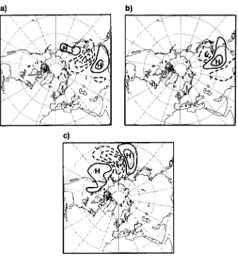
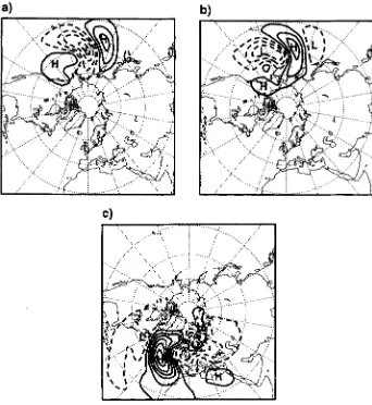
VECTORS 1699

Figure 1 . Stream-function fields of the three leading initial total-energy singular vectors at 500 hPa for 0000

zyxwvutsrqponmlkjihgfedcbaZYXWVUTSRQPONMLKJIHGFEDCBA

UTC

1 November 1995 and an optimization time of one day. Solid (dashed) lines denote positive (negative) values and

the contour interval is 5

x rn2s-l.

algorithm (Strang 1986). Palmer et al.

(1998) study the impact of choosing different simple

metrics at initial time, keeping the total energy metric at optimization time. The spectra of the singular vectors can differ substantially for the various metrics. It turns out that, of the simple metrics considered, the total energy metric is the most consistent with the analysis-error statistics.

To study the impact of the analysis-error covariance metric on the singular vectors

we used a five-level version of the ECMWF Integrating Forecast System model (Simmons

zyxwvutsrqponmlkjihgfedcbaZYXWVUTSRQPONMLKJIHGFEDCBA

et al. 1989; Courtier et al. 1991) with a triangular truncation at wave number 21 and a simple vertical diffusion scheme (Buizza 1994). The model levels are at 100,300,500,700 and 900 hPa. The initial time for the singular vector computation is 0000 UTC 1 November

1995 and the optimization time is one day.

(6)

1700

J. BARKMEIJER

zyxwvutsrqponmlkjihgfedcbaZYXWVUTSRQPONMLKJIHGFEDCBA

et

al.

z

2i

54-

0

. .

5 10

I

,’

@

-

15 20 25 30

Total energy

1

35 40

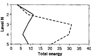
Figure 2. Vertical cross-section of the total-energy distribution of the ten leading total-energy singular vectors with respect to the five model levels. The dashed line represents the initial profile and the solid line represents the

energy after

zyxwvutsrqponmlkjihgfedcbaZYXWVUTSRQPONMLKJIHGFEDCBA

24 hours of linear integration. The energy in rn’s-’ at initial and final time has been multiplied by factors of 100 and 5 respectively.

is located over the Pacific. The vertical distributions of energy in the singular vectors at initial and optimization time are given in Fig. 2. It shows that the energy at initial time is confined to near the baroclinic steering level. During time evolution the energy propagates upwards and downwards, indicating error growth (Buizza and Palmer 1995).

When C is specified to be equal to the full Hessian of the 3D-Var cost function, the operator C is not known in matrix form, and determining its square root is not feasible. In order to solve (9), a generalized eigenvalue problem solver, called the generalized Davidson method, is used (see appendix). This algorithm can solve (9) efficiently and requires only the ability to calculate y = Sx, where S is any of the operators M, P, E and C. No explicit knowledge of any operator is needed. In the following we assume that the total energy metric is always used at optimization time.

To improve the performance of the generalized Davidson algorithm, a coordinate transformation ,y = L-’x was carried out with LLT = B. Applying the transformation L,

the Hessian becomes equal to the sum of the identity and a matrix of rank less than or equal to the dimension of the vector of observations (see also Fisher and Courtier (1995)). Thus, when no observations are used in the cost function, the transformed operator (L-’)TCL-l

is the identity, and the proposed algorithm is equivalent to the Lanczos algorithm (see appendix). Observe that a similar coordinate transformation was used to compute the TESVs. Defining singular vectors using the total energy metric at initial time may be interpreted as using a background-error covariance matrix B with the assumption of no

horizontal and vertical correlation of forecast error.

( a ) Univariate background-error covariance matrix

[image:6.486.162.322.61.159.2]

(7)

SINGULAR VECTORS

1701

Figure 3. Same as Fig. I but for the Hessian singular vectors without observations.

zyxwvutsrqponmlkjihgfedcbaZYXWVUTSRQPONMLKJIHGFEDCBA

0

5 10

15

20 25 30 35 40

Total energy

[image:7.486.73.418.80.462.2]

(8)

1702

zyxwvutsrqponmlkjihgfedcbaZYXWVUTSRQPONMLKJIHGFEDCBA

J. BARKMEIJER et

al.

3.5 -

3 -

0

m 2.5 -

C 0

‘3 2 -

Q

0 z

E 1 . 5 -

E

a

1 -

L, c

r

.-

0.5 0

1

0 1 2 3 4 5

6

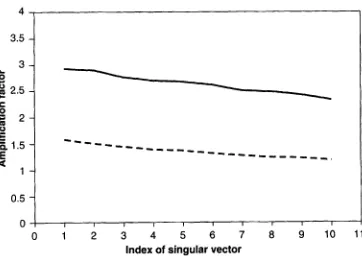
7 8 9 1 0 1 1 [image:8.486.60.422.60.318.2]

Index of singular vector

Figure 5 . Amplification factor of the ten leading total-energy singular vectors (solid line) and Hessian singular vectors without observations (dashed line), as given by the square root of the ratio between the total energy at final

and initial time.

forecast differences) reaches a maximum near the jet level, and this is reflected in the metric defined by the Hessian. Also, the background-error covariance matrix is specified to have broad horizontal and vertical correlations, and thus penalizes the occurrence of baroclinic structures in the analysis error. Hence we may suspect that the 3D-Var Hessian metric penalizes the sharp and baroclinic error patterns too much in the areas which are picked up by the singular vector computation.

Another way to highlight the differences between the TESVs and HSVs is to determine the similarity index of two unstable subspaces (Buizza 1994). To that end a Gram-Schmidt procedure is applied to the first ten TESVs and HSVs at initial time. Denote by WH and

WTE the space thus obtained in the case of the HSVs and TESVs, respectively:

(1 1 )

WTE)

w ~ ( ~ ~ )

= span{vj , j = I ,

.

. .

10).

The similarity index

9’

zyxwvutsrqponmlkjihgfedcbaZYXWVUTSRQPONMLKJIHGFEDCBA

of the two unstable subspaces WH and WE is then defined by

I i n

Y(WH, WTE) =

-L

2

(VY, v y ) 2 , lo j , k = l

where (

,

) is the inner product associated with the total-energy norm. The similarity index

(9)

SINGULAR VECTORS

zyxwvutsrqponmlkjihgfedcbaZYXWVUTSRQPONMLKJIHGFEDCBA

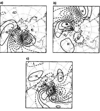
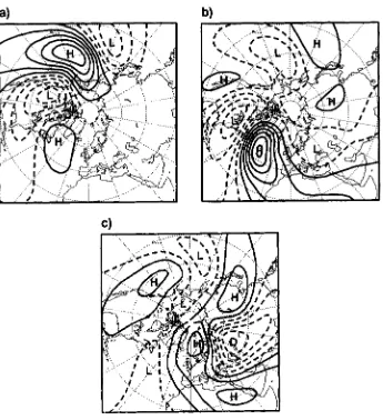
1703 The impact of observational locations and errors on the HSVs was studied using

covariance information from most of the conventional observations (SYNOP, AIREP,

SATOB, DRIBU, TEMP, PILOT, SATEM and PAOB) from two areas: EUR (2WW-20"E;

30"N-80°N) and PAC ( 17OoW-13O0w, 3O0N-80"N). Figures 6(a)-(c) show the first three HSVs at 500 hPa using observations from EUR. Compared to the HSVs without observations (Fig. 3), the amplitudes of the leading HSVs over EUR have decreased substantially. Including observational-error statistics left the vertical structure of the HSV basically un- altered (not shown). The similarity index of the two unstable subspaces, i.e. formed by HSVs computed with and without covariance information of observations from EUR, and spanned by the ten leading HSVs, is 0.79. Repeating the same for PAC gave similar results (see Figs. 6(d)-(f)). The amplitude of the SVs is now reduced over the PAC area at initial time. A comparison of the two unstable subspaces computed in the same way as the EUR

yields a similarity index of 0.73.

zyxwvutsrqponmlkjihgfedcbaZYXWVUTSRQPONMLKJIHGFEDCBA

(b) Total-energy background covariance matrix with observations

In order to investigate the impact of covariance information from observations on the TESVs, the 3D-Var background-error covariance matrix in the generalized eigenvalue calculation (9) was modified to a diagonal matrix whose diagonal contained the reciprocal of the total-energy weights (see (10)). The SVs are now computed in terms of the control

variable

x

zyxwvutsrqponmlkjihgfedcbaZYXWVUTSRQPONMLKJIHGFEDCBA

and we checked that, without observations, the same SVs resulted in terms of

the model variables as defined by (9).

The SVs computed without observations do not depend on the scaling of the background covariance matrix. However, in order to account reasonably well for the way the observations are used in the 3D-Var analysis procedure, one needs to ensure that the relative magnitude of the background- and observation-error variances is balanced. Performing an analysis procedure with the modified background covariance matrix should give analysis increments which are consistent with the amplitude of the operational analysis increments. The appropriate magnitude of the total-energy background-error covariance matrix was determined by computing the analysis increments at a particular observation point for different scalings of the matrix and selecting one that implies sensible amplitudes for the increments.

In the 3D-Var analysis procedure, the analysis increments, x" - x', are a linear combination of the observation increments, y - Hxb, (Lorenc 1986; (A.9)):

xa - xb = BHT(HBHT

+

R)-'(y - Hx'), (13)

where H is the linearization of the observation operator H in the vicinity of the background xb. In the case of one observation, HT reduces to a vector hT of the same dimension as

the model state vector, and the specified background error :

zyxwvutsrqponmlkjihgfedcbaZYXWVUTSRQPONMLKJIHGFEDCBA

a for the observed parameter

satisfies CT; = hBhT. Denoting the observation variance by :,a (13) can be written as

b y - H x b

x a - x = B h

(

) .

+

u:

Applying h to both sides of (14) yields for the analysis increments at the observation point h(xa - xb) = hBhT

(

y - Hx' 2 ) =

("-)

(y - HXb),

0; +a, a:

+

u,'

Using the linearization H of the observation operator in the vicinity of the background, we may write to first order

(16)

(10)

[image:10.486.65.416.68.626.2]

1704

J.

zyxwvutsrqponmlkjihgfedcbaZYXWVUTSRQPONMLKJIHGFEDCBA

BARKMEIJER et

al.

... : . . . - . . . ... ; _....

I

... . .

, ..

. . .. .

'a, . ; . . . _. _.

. .

a

. : _{. .}_{. .} .

Figure 6. Same as Fig.

zyxwvutsrqponmlkjihgfedcbaZYXWVUTSRQPONMLKJIHGFEDCBA

3 but for Hessian singular vectors with observations from (a)-(c) EUR (20"W-2OoE;

(11)

[image:11.486.71.413.61.433.2] [image:11.486.153.334.509.538.2]

SINGULAR VECTORS

zyxwvutsrqponmlkjihgfedcbaZYXWVUTSRQPONMLKJIHGFEDCBA

1705

Figure 7. Same as Fig. 1 but now with observations from the northern hemisphere extratropics.

Combining (15) and (16) we obtain

at, 2

=a: (-),withr= r

Hx" - Hxh

1 - r y - H x b '

To determine the appropriate magnitude of the variances in B, a 3D-Var minimization

was performed using error statistics of only one observation. The scaling of B was tuned

so that the a h estimated from (17) is approximately equal to

zyxwvutsrqponmlkjihgfedcbaZYXWVUTSRQPONMLKJIHGFEDCBA

0, in the case of an AIREP

observation of temperature at 500 hPa (a, = 2 K). These values for a, and a h are assumed

to be reasonable approximations of actual errors for temperature in the areas of interest for the SVs.

Figure 7 shows the three leading TESVs when covariance information of observations is included in the computation. The same type of observations are used as for PAC and EUR but now for the northern hemisphere extratropics (3OoN-90"N). Observe that the

(12)

I706 J. BARKMEIJER

zyxwvutsrqponmlkjihgfedcbaZYXWVUTSRQPONMLKJIHGFEDCBA

et al.

are from satellites, which have less weight in the 3D-Var cost function than conventional

data. Comparing these

SVs with the TESVs when no observational information is used

(see Fig. 1) yields a similarity index of 0.5. We conclude that incorporating statistics of

observational errors in the SV computation may change the unstable subspace considerably.

4. APPROXIMATION OF THE HESSIAN

A possible alternative to using a generalized eigenvalue problem solver is to replace

the full Hessian B-I

zyxwvutsrqponmlkjihgfedcbaZYXWVUTSRQPONMLKJIHGFEDCBA

+

HTR-'H (see

(4)) by an approximating operator which can easily

be inverted. In this way, solving a generalized eigenvalue problem can be reduced to solving an ordinary eigenvalue problem. As noted in section 3, the Hessian in terms of the control vector ,y = L-'x is the sum of the identity I and a matrix of rank less than or equal to the

number of observations, and can be written as (see also Fisher and Courtier 1995):

where

zyxwvutsrqponmlkjihgfedcbaZYXWVUTSRQPONMLKJIHGFEDCBA

hi and ui are eigenpairs of the Hessian and K denotes the number of obser-

vations. Observe that indeed {I

+

Cf=l(hi

- l)uiuT}uk = uk

+

(Ak - l)uk = hkuk, for

k = 1 ,

. . .

K , because of the orthogonality of the eigenvectors ui. Since the Hessian can

be written in the form (18), the square root of the inverse of the Hessian can be readily

determined using the Sherman-Momson and Woodbury formula (Wait 1979) and it is

given by

Multiplying both sides of (9) to the left and right with the above operator yields an eigen-

value problem which again can be solved with the Lanczos algorithm.

We consider two situations to see how well SVs with an approximated Hessian com-

pared to SVs obtained without approximation of the Hessian. In the first experiment (El)

the full background covariance matrix B was used together with covariance information

for observations from EUR. In the second experiment (E2) a diagonal background-error covariance matrix was used with the inverse of the total-energy weights as variances and with observational statistics for observations from the northern hemisphere extratropics. The same observation sets are used as in section 3(a). Table 1 gives, for each experiment E l and E2, the similarity index between the unstable subspace formed by the leading ten SVs thus obtained and the SVs in the case where the Hessian is approximated by 100 or

150 eigenvectors. Clearly, the leading singular vectors computed with an approximated

TABLE 1 . SIMILARITY INDICES BETWEEN IMENTS, WITH THE HESSIAN APPROXIMATED

USING 100 AND 150 EIGENPAIRS.

Number of eigenpairs used 100 150

THE UNSTABLE SUBSPACES FOR TWO EXPER-

Experiment El 0.71 0.83 Experiment E2 0.63 0.14

(13)

SINGULAR VECTORS

1707

Figure 8. Stream-function fields at 500 hPa of the three leading Hessian singular vectors using 150 eigenpairs in the approximation of the Hessian and observations from EUR (20"W-20°E 30"N-80'"). Solid (dashed) lines

denote positive (negative) values and the contour interval is 5

x lo-* m's-'.

Hessian, based on 150 eigenpairs, capture reasonably well the dominant part of the unstable subspace obtained with the full Hessian. Figure 8 shows the stream-function fields at

500 hPa of the first three singular vector for experiment El. In particular, the first singular vector compares well with the corresponding HSV computed with the full Hessian (see

Fig. 6(a)).

zyxwvutsrqponmlkjihgfedcbaZYXWVUTSRQPONMLKJIHGFEDCBA

5. FINAL REMARKS

[image:13.486.74.419.60.438.2]

(14)

1708

zyxwvutsrqponmlkjihgfedcbaZYXWVUTSRQPONMLKJIHGFEDCBA

J. BARKMEIJER

et al.

analysis-error covariance metric) to determine singular vectors is that it requires an efficient solution of a generalized eigenvalue problem. Because of the difficulty of solving such a system, the calculation of singular vectors up to now has been based on an energy metric, which may be interpreted as an approximation of the analysis-error statistics (Palmer

et al. 1998). With this approximation, the singular vectors can be efficiently computed by applying the Lanczos algorithm to the propagators of the tangent and adjoint model.

The method described in this paper uses the full Hessian (or second derivative) of the cost function of the variational data assimilation as an approximation to the analysis-error covariance metric. In this way the calculation of singular vectors can be made consistent with the 3D/4D-Var calculation of the analysed state. The algorithm to solve the generalized eigenproblem is a generalization of the Davidson algorithm (Davidson 1975). It requires only that the propagators of the linear and adjoint model and the Hessian of the cost

function are available in operator form, i.e. y

zyxwvutsrqponmlkjihgfedcbaZYXWVUTSRQPONMLKJIHGFEDCBA

= Sx

can be computed, where S is any of

these operators and

x

is an input vector.

We used the Hessian from different configurations of the 3D-Var cost function. When no observations are used in 3D-Var, the analysis-error metric is entirely based on the description of the first-guess error. Currently the first-guess error statistics are derived from the difference between the two-day and one-day forecast valid for the same day (the so-called NMC method, Parrish and Derber (1992)). The background covariance matrix defined in this way penalizes the occurrence of baroclinic structures in the analysis error and it lacks a realistic description of small-scale error structures. Experiments with a five- level PE model gave singular vectors which are of larger scale than the singular vectors defined in terms of the total-energy metric. Also, the vertical structure of the singular vectors revealed a difference with respect to the energy distribution. Most of the energy is confined to the upper levels when the Hessian was used, instead of peaking around the baroclinic steering level as in the case of total-energy singular vectors. Including covariance information of observations in the Hessian mainly changed the location of the maxima of the singular vectors. The amplitude of the singular vectors was reduced substantially over the areas where observations were present.

The impact of observational-error statistics on the singular vectors which are used in the ECMWF EPS was investigated by modifying the background-error covariance matrix. By setting this matrix to a diagonal matrix with the inverse of the total-energy weights on its diagonal, the total-energy singular vectors are retrieved when no observations are used. Using most of the conventional observations from the northern hemisphere extratropics leads to a significant change of the unstable subspace as spanned by the leading singular vectors. This may have consequences for the set-up of future observational experiments such as Fronts and Atlantic Storm Tracks Experiment. The areas to perform adaptive observations as indicated by the leading singular vectors may change when statistics of observational errors are included in the singular-vector computation.

Although the proposed algorithm is of the order of three times more expensive computationally than the Lanczos algorithm, there is scope to improve upon this. One way is to reduce the number of observations without essentially changing the 3D-Var analysis procedure. Another possibility would be to approximate the Hessian through its leading eigenpairs. By doing so, the Lanczos algorithm can again be used to determine singular vectors. Preliminary experiments showed that by using a considerable number (150) of eigenpairs in the approximation of the Hessian, the dominant part of the unstable subspace could be reasonably well retrieved. The additional computation time needed to determine 150 eigenpairs of the Hessian is around 10% of the time to solve the Lanczos problem.

(15)

SINGULAR VECTORS 1709

and full-background covariance matrix indicate that some effort must be put into correctly modelling the background error. It seems that neither the 3D-Var nor the total-energy background-error metric are completely satisfactory for the calculation of singular vectors: the implied correlation structure seems respectively, either too broad or too sharp. A first improvement would be to optimize the 3D-Var background-error term for areas which are pointed to by the singular vectors. One can also use the 4D-Var Hessian. A definite answer to the problem will only come when some flow-dependent error covariances are estimated using a simplified Kalman filter. These approaches are being tried at ECMW.

ACKNOWLEDGEMENTS

We thank R. Buizza, T. Palmer and M. Fisher for the stimulating discussions we had during the preparation of this paper, The advice from H. A. van der Vorst and G. L. G. Sleijpen on solving the generalized eigenvalue problem was very helpful. Also thanks are due to A. Hollingsworth and A. Simmons for carefully reading the manuscript. Finally the comments given by two reviewers were much appreciated.

APPENDIX

The generalized eigenproblem

is usually handled by bringing it back to a standard eigenproblem

The matrix B-IA is in general non-symmetric, even if both A and B are symmetric.

However, if

zyxwvutsrqponmlkjihgfedcbaZYXWVUTSRQPONMLKJIHGFEDCBA

3 is symmetric and positive definite, the B inner product is well defined. The

matrix B-'A is symmetric in this inner product if A. is symmetric:

(w, B-'Av)B

= (Bw, B-'Av) = (w, Av) = (Aw, V) = (B-lAw, V)B, (A.3) where w and v are arbitrary vectors. The proposed method to solve (A.l) constructs a set of

basis vectors V of a search space "Ir, cf. the Lanczos method (Lanczos 1950; Strang 1986). The approximate eigenvectors are linear combinations of the vectors V. The classical and most natural choice for the search space 'V, for instance utilized in the Lanczos method, is the so-called Krylov subspace, the space spanned by the vectors

V, B-'AV, (B-'A)~V,

. .

.

, ( B - ~ A ) ~ - ~ v . 64.4) This i-dimensional subspace is denoted by SC'(v, B-IA). The vector v is a starting vector

that has to be chosen. The Krylov subspace is well suited for computing dominant eigenpairs since the vector (B-'A)'-'v has a (much) larger component in the direction of the dominant eigenvector than v.

In the next three subsections we will discuss how approximate eigenpairs can be computed from a given subspace, how a B-orthogonal basis for the Krylov subspace can be constructed, and how operations with B-' can be avoided in the construction of the basis. This last subject is of particular importance in our application, since we have no

(16)

1710

zyxwvutsrqponmlkjihgfedcbaZYXWVUTSRQPONMLKJIHGFEDCBA

J. BARKMEIJER

et al.

How to compute approximate eigenpairs

Given a search space 'V the approximate eigenpair (0, u) is a linear combination of the basis vectors of 7 f :

u = v y . (A.5)

A suitable criterion for finding an optimal pair (0, u) is the Galerkin condition that (A.6)

the residual

r = B - ~ A U - ou = B-~AVY - OVY is B-orthogonal to the search space V. Hence

VTBr = 0 64.7)

and consequently, using (A.6),

Note that the resulting eigenproblem is of the dimension of the search space, which is generally much smaller than that of the original problem. The basis vectors are usually orthogonalized so that VTBV = I. Approximate eigenpairs that adhere to the Galerkin

condition are called Ritz pairs.

Construction of a basis for the Krylov subspace

If approximate eigenpairs are computed according to (A.8), then the residuals r l ,

r2,

. . .

, ri form a B-orthogonal basis for

X i

zyxwvutsrqponmlkjihgfedcbaZYXWVUTSRQPONMLKJIHGFEDCBA

(rl ,B-'A). The B-orthogonality

rTBrj = 0 (A.9)

of the residuals ri follows immediately from their construction. According to (A.8) it is true

for i < j .

Since B is symmetric the inner product is symmetric in i and j , and consequently

it also holds for i > j .

It remains to show that the residuals form a basis for this Krylov subspace. Given a (i - 1)-dimensional search space, the Galerkin condition (A.8) yields i - 1 approximate eigenpairs and residuals. The search space can be extended with any of these residuals. Each selected residual ri will be a new B-orthogonal basis vector for

X i

(v, B-lA):

span{rl, r2,

.

. .

, ri) = Y ( r l , B-~A). (A. 10) This can be seen by noting that the residual is given by (see (A.6))

ri = B - ~ A U ~ - ~ -ei-,ui-, = B - ' A V ~ - ~ ~ ~ - ~ -Oi-lvi-,yi-l, (A.11)

with (Oi-l,

zyxwvutsrqponmlkjihgfedcbaZYXWVUTSRQPONMLKJIHGFEDCBA

uiP1) an eigenpair approximation in the space Xi-'(r1, B-IA). Since

B - ~ A v ~ - ~ ~ ~ - ~

E YC(rl, B - ~ A ) , (A. 12)

the residual ri also belongs to

Yc'

(rl , B-'A). Because ri cannot be expressed as a linear

(17)

SINGULAR

VECTORS

1711

Solution method

As was stated before, the natural search space for the generalized eigenvalue problem

is the Krylov subspace

YC;

(v, B-'A). This basis can be generated by expanding the basis

by new residual vectors. The problem in the construction of a basis for this space is that operations with

B-'

are needed. Since in our application the inverse of

B

is not known explicitly, we approximated its action by an iterative solution method, like the Conjugate Gradient method (CG) (Hestenes and Stiefel 1954) or the Conjugate Residual method (CR) (Cline 1976). To compute the vector

r = B-'F, (A.13) one iteratively solves the system

B r = ?. (A.14)

Iterative solution methods require, apart from vector operations, only multiplications with B. The vector r can in principle be determined to high accuracy. This, however, may require many multiplications with B and hence may be very expensive. We therefore propose to approximate the action of B to low accuracy only, by performing only a few steps with an iterative solution method. The subspace generated in this way is not a Krylov subspace and the basis vectors are not the residuals (A.6) but only approximations to it. As a consequence they are not perfectly B-orthogonal. Orthogonality has to be enforced explicitly.

The algorithm we use can be summarized as follows:

zyxwvutsrqponmlkjihgfedcbaZYXWVUTSRQPONMLKJIHGFEDCBA

0 Select number of CR steps, maximum dimension of

V,

starting vector v. 0 Compute Bv, B-normalize v.

0 Do

i = 1 until maximum dimension of V:

1. compute

AV,

VTAV,

2. solve small eigenproblem

VTAVy

= By,

3. select y. Ritz value 8,

4. compute Ritz vector u =

Vy

and residual F =

AVy

- BBVy,

5. compute approximately v = B-'? with the CR method, 6. B-orthonormalize new v against

V,

7. expand

V

with the resulting vector.

The matrix V contains the basis for the search space, the vector v contains the new

basis vector, and (u, 0) is an approximate eigenpair. In step 3 the pair with the largest

zyxwvutsrqponmlkjihgfedcbaZYXWVUTSRQPONMLKJIHGFEDCBA

8 is

selected since we are interested in the upper part of the spectrum. However, if the eigenpair

approximation reaches a certain accuracy E , i.e.

?

= Au - 8Bu G

E , a smaller 8 is selected.

In step 5 a few CR steps are performed to approximate the action of BPI. Another iterative

solution, e.g. CG, could also be used. The optimal number of CR iterations depends mainly on the cost of operations with B. If these are expensive the number of CR iterations should be kept small. In our experiments the number of CR steps per iteration is 15. Evaluation of

A and B is then computationally equally expensive. In step 6 the modified Gram-Schmidt

procedure is used for reasons of numerical stability.

Relation with standard methods

The above method is closely related to Davidson's method (Davidson 1975) for solving the standard eigenproblem. The difference is that we try to approximate B-' by means of an iterative solution method, whereas in Davidson's method the action of (A - BI)-' is

(18)

1712 J. BARKMEIJER

zyxwvutsrqponmlkjihgfedcbaZYXWVUTSRQPONMLKJIHGFEDCBA

e t al.

on Galerkin approximations for the eigenpairs. Recently, an improvement over David- son's method has been proposed by Sleijpen and Van der Vorst (1996), the so called Jacobi-Davidson method. The essential difference between the Davidson method and the

Jacobi-Davidson method is that in the latter the action of

(A

- OI)-' is approximated in the

space orthogonal to the Ritz vector u. Sleijpen et

zyxwvutsrqponmlkjihgfedcbaZYXWVUTSRQPONMLKJIHGFEDCBA

al. (1996) give a framework for Davidson

and Jacobi-Davidson type methods to solve generalized and polynomial eigenproblems. The method described above can be seen as a generalized Davidson method. If the action of B-' is approximated to machine accuracy, or if B = I, the eigenpair approximations

should be the same as the ones obtained with the Lanczos method.

Bouttier, F. Buizza, R.

Buizza, R. and Palmer, T. N. Cline. A. K.

Courtier, P., Freyder, C.,

Geleyn, J.

zyxwvutsrqponmlkjihgfedcbaZYXWVUTSRQPONMLKJIHGFEDCBA

F., Rabier, F. and Rochas, M.

Heckley, W., Pailleux, J., VasiljeviC, D., Hamrud, M., Hollingsworth, A., Rabier, E and Fisher, M.

Courtier, P., Andersson, E., Davidson, E. R.

Ehrendorfer, M. and Tribbia, J. J. Epstein, E. S.

Fisher, M. and Courtier, P. Hestenes, M. R. and Stiefel, E. Houtekamer, P. L.

Houtekamer, P. L., Lefaivre, L., Derome, J., Ritchie, H. and Mitchell, H. L.

Lanczos, C. Leith, C. E. Lorenc, A. C. Lorenz, E. N.

Mardia, K. V., Kent, J. T. and Bibby, J. M.

Molteni, F., Buizza, R., Palmer, T. N. and

Petroliagis, T. 1994 1994 1995 1995 1976 1991 1998 1975 1997 1969 1995 I954 1995 1996 1950 1974 1986 1965 1979 1996 REFERENCES

A dynamical estimation of error covariances in an assimilation system. Mvn. Weather Rev., 122,2376-2390

Sensitivity of optimal unstable structures. Q. J. R. Meteorol. Svc.,

120,429-45 1

Optimal perturbation time evolution and sensitivity of ensemble

prediction to perturbation amplitude. Q. J. R. Metevrvl. Soc.,

zyxwvutsrqponmlkjihgfedcbaZYXWVUTSRQPONMLKJIHGFEDCBA

The singular vector structure of the atmospheric general circula- tion. J. Atmvs. Sci., 52, 1434-1456

Several observations on the use of conjugate gradient methods. ICASE Report 76, NASA Langley Research Center, Hamp- ton, Virginia, USA

'The Arpege project at MCtCo France'. Proceedings of ECMWF seminar on numerical methods in atmospheric models, 9-13 September 1991, Vol. 2. ECMWF, Reading, UK

The ECMWF implementation of three-dimensional variational assimilation (3D-Var). Part I Formulation. Q. J. R. Metevrul.

Svc., (in press)

121,1705-1738

The iterative calculation of a few of the lowest eigenvalues and corresponding eigenvectors of large real symmetric matrices.

J. Cvmp. Phys., 17,87-94

Optimal prediction of forecast error covariances through singular vectors. J. Atmvs. Sci., 54,286313

Stochastic dynamic predictions. Tellus, 21,739-759

Estimating the covariance matrices of analysis and forecast error

in variational data assimilation. ECMWF, Technical Memo-

randum No. 220

Methods of conjugate gradients for solving linear systems. J. Res. Nat. Bur. Stand., 49,409436

The construction of optimal modes. Mvn. Weather Rev., 122,

A system approach to ensemble prediction. Mvn. Weather Rev., 21 79-21 9 1

124,1225-1242

An iteration method for the solution of the eigenvalue problem

of linear differential and integral operators. J. Res. Nat. Bur. Stand., 45,255-282

Theoretical skill of Monte Carlo forecasts. Mvn. Weather Rev., 102,4094 18

Analysis methods for numerical weather prediction.

Q. J. R. Metevrvl. Svc., 112, 1177-1194

A study of the predictability of a 28-variable atmospheric model.

Tellus, 17,321-333

Multivariate analysis. Academic Press, London

(19)

SINGULAR VECTORS 1713 Palmer, T. N., Gelaro, R.,

Parrish, D. I. and Derber, J. C.

Rabier, F. and Courtier, I?

zyxwvutsrqponmlkjihgfedcbaZYXWVUTSRQPONMLKJIHGFEDCBA

Rabier, F., Klinker, E., Courtier, P. and Hollingsworth, A. Rabier, F., McNally, A.,

Anderson, E., Courtier, P., UndCn, P., Eyre, J.,

Hollingsworth, A.

and Bouttier, F.

Simmons, A. J., Bumdge, D. M., Jarraud, M., Girard, M. and Wergen, W.

Vorst, H. A.

Fokkema, D. R. and van der Vorst, H. A.

Barkmeijer, J. and Buizza, R.

Sleijpen, G. L. G. and van der

Sleijpen, G. L. G., Booten, J.

zyxwvutsrqponmlkjihgfedcbaZYXWVUTSRQPONMLKJIHGFEDCBA

G . L., Stephenson, D. B.

Strang, G.

ThBpaut, J.-N., Courtier, P., Belaud, G. and Lemaitre, G .

Toth, Z. and Kalnay, E. Van den Dool, H. M. and

Rukhovets, L. Wait, R. 1998 1992 1992 1996 1998 1989 1996 1996 1997 1986 1996 1997 1994 1979

Singular vectors, metrics and adaptive observations. J. Atmos. Sci.,

54,633-653

The National Meteorological Centre’s spectral statistical interpo- lation analysis system. Mon. Weather Rev., 120, 1740-1763 Four-dimensional assimilation in the presence of baroclinic insta-

bility. Q. J. R . Meteorol. Soc., 118,649-672

Sensitivity of forecast errors to initial conditions. Q. J. R. Meteorol.

The ECMWF implementation of three-dimensional variational assimilation (3D-Var). Part I 1 Structure functions. Q . J. R. Meteorol. Soc., (in press)

Soc., 122,121-150

The ECMWF medium-range prediction models development of the numerical formulations and the impact of increased resolution. Meteorol. Atmos. Phys., 40,28-60

A Jacobi-Davidson iteration method for linear eigenvalue prob-

lems. SIAM J. Matrix Anal. Appl., 17,401-425

Jacobi-Davidson type methods for generalized eigenproblems and polynomial eigenproblems. BIT, 36,595433

Correlation of spatial climate/weather maps and the advantages of using the Mahalanobis metric in predictions. Tellus, 49A,

Introduction to applied mathematics. Wellesley-Cambridge Press Dynamical structure functions in a four-dimensional variational assimilation: A case-study. Q. J. R. Meteorol. Soc., 122,535- 561

Ensemble forecasting

zyxwvutsrqponmlkjihgfedcbaZYXWVUTSRQPONMLKJIHGFEDCBA

at NCEP and the breeding method. Mon.

Weather Rev., 125,3297-3319

On the weights for an ensemble-averaged 6-10-day forecast.

Weather Forecasting, 9,457-565

The numerical solution ofalgebraic equations. John Wiley &

Sons,