Pemodelan Celular Automata Untuk Visualisasi Dan Prediksi Pola Penyebaran Penyakit Demam Berdarah.

(1)

A CELLULAR AUTOMATA MODELING FOR VISUALIZING

AND PREDICTING SPREADING PATTERNS

OF DENGUE FEVER

PUSPA EOSINA HOSEN

GRADUATE SCHOOL

BOGOR AGRICULTURAL UNIVERSITY BOGOR

(2)

(3)

STATEMENT OF THESIS AND SOURCES OF

INFORMATION AND DEVOLUTION COPYRIGHT

Hereby, I state that the thesis entitled “A Cellular Automata Modeling for Visualizing and Predicting Spreading Patterns of Dengue Fever” is my own work and to the best of my knowledge, under supervision by Dr Eng Taufik Djatna, STP MSi and Helda Khusun, STP MSc PhD. It has never previously been published in any university. All of incorporated originated from other published as well as unpublished papers are stated clearly in the texts as well as in the references.

Hereby, I devolve the copyright of my thesis to Bogor Agricultural University.

Bogor, August 2015

Puspa Eosina Hosen

(4)

SUMMARY

PUSPA EOSINA HOSEN. A Cellular Automata Modeling for Visualizing and Predicting Spreading Patterns of Dengue Fever. Supervised by TAUFIK DJATNA and HELDA KHUSUN.

Modeling is a simplification of a real problem, aiming to study and understand the phenomena in the real world. In epidemiology, system modeling approach is commonly used for viewing the epidemic process. Moreover, visualization is required as the first step in epidemiological analysis to understand the spatial characteristics of a dataset, identifying the epidemiology of disease pattern in a given geographical area, predicting the spreading pattern of disease in the next period. Unfortunately, Ordinary Differential Equation (ODE) or statistical models the most common method used in epidemiological analysis are unable to elaborate spatial patterns and interactions such as in visualization and prediction of spreading disease. This limitation could be overcome by using Cellular Automata (CA) model.

The use of CA models in many problems such as in epidemic process analysis and spatiotemporal pattern analysis showed the powerful of CA in solving the problem that related to the spatial pattern. CA is one of the dynamic system approaches that implementing discretization of time and space. CA consists of cells, called cellular space, a local connection to other cells, and boundary conditions. Each cell, representing a state, could change at every time-step using local transmission rules which generate a new state based on the previous state of the cell and its neighborhood. Therefore, the concept of neighborhood is very important. The other important aspect that determines the accuracy of CA model is the trasmition rule f. This rule is able to be represented as a deterministic or probabilistic function.

In this research, we proposed a new approach in developing a spreading pattern model of Dengue Hemorrhagic Fever (DHF) based on CA. We especially focused on determining a probabilistic function using Hidden Markov Model (HMM) which has not been used by researchers yet. HMM is a probabilistic model that is suitable for solving the problem related to the sequential-temporal data. To show the effectiveness of the proposed model, we implemented this approach to the DHF case. We used dataset from a limited area such as West Bogor in the period of 2013 and defined the state criteria from these dataset. Moreover, we only considered an infective state which was dedicated particular attention to the spatial distribution of infected areas. The evaluation was conducted by comparing the results of data simulation of the proposed model to that of one yielded by the Susceptible-Infected-Recovered (SIR) model, as a classical approach. The evaluation result showed that the CA model was capable of generating patterns that similar to the patterns generated by SIR models with a similarities value of 0.95.

(5)

RINGKASAN

PUSPA EOSINA HOSEN. Pemodelan Celular Automata untuk Visualisasi dan Prediksi Pola Penyebaran Penyakit Demam Berdarah. Supervised by TAUFIK DJATNA and HELDA KHUSUN.

Pemodelan adalah penyederhaan dari sebuah masalah atau fenomena di dunia nyata yang bertujuan untuk mempelajari dan memahaminya. Pada epidemiologi, pemodelan pada umumnya digunakan untuk melihat proses epidemik. Oleh karena itu, visualisasi diperlukan sebagai langkah awal, antara lain pada analisis epidemiologi untuk memahami karakter spasial dari dataset, mengidentifikasi pola penyebaran penyakit pada area geografis tertentu, dan memprediksi pola penyebaran penyakit pada periode selanjutnya. Selama ini,

Ordinary Diferential Equation (ODE) atau statistik, sebagai model yang paling umum digunakan pada analisis epidemiologi, tidak dapat mengelaborasi proses dari pola spasial dan interaksinya, seperti pada kasus visualisasi dan prediksi penyebaran penyakit. Model Cellular Automata (CA) diperkenalkan sebagai model yang dapat mengatasi keterbatasan dari model ODE dan statistik tersebut.

Penggunaan model CA pada banyak kasus, seperti analisis proses epidemik dan analisis pola spatio-temporal memperlihatkan CA cukup baik dalam memecahkan permalahan yang berkaitan dengan pola spasial. Model CA adalah pendekatan sistem dinamik yang mengimplementasikan konsep diskritasi ruang dan waktu. Model ini terdiri atas sel-sel yang disebar pada ruang selular, sebuah koneksi lokal yang menghubungkan sel yang satu dengan sel yang lain, serta kondisi batas. Setiap sel berada pada nilai state tertentu yang dapat berubah ke nilai state lain setiap waktu. Perubahan state dipengaruhi oleh state sel tersebut dan lingkungannya (neighborhood) pada periode sebelumnya. Oleh karena itu, konsep neighborhood menjadi penting. Aspek penting lainnya yang menentukan akurasi model CA adalah aturan trasmisi perubahan state untuk setiap sel yang merupakan sebuah fungsi yang bersifat probabilistik.

Pada penelitian ini, diusulkan suatu pendekatan dalam mengembangkan model penyebaran penyakit Demam Berdarah Dengue (DBD) berbasis CA. Penelitian ini difokuskan pada penentuan fungsi probabilisitik, sebagai CA rule, menggunakan pendekatan Hidden Markov Model (HMM) yang belum pernah digunakan oleh peneliti-peneliti sebelumnya untuk model CA. HMM adalah model probabilistik yang sesuai untuk memecahkan permasalahan data sekuensial temporal. Untuk memperlihatkan efektivitas model yang diusulkan, pendekatan ini diimplementasikan pada kasus DBD di wilayah Bogor Barat tahun 2013. Dari

dataset ini didefinisikan beberapa kriteria state untuk memodelkan proses spasial kondisi terinfeksi (infective state) kelurahan-kelurahan di Bogor Barat. Evaluasi dilakukan dengan membandingkan hasil simulasi data dari model yang diusulkan terhadap hasil simulasi data yang diperoleh dari model Susceptible-Infected-Recovered (SIR), yaitu salah satu pendekatan klasik yang paling sering digunakan dalam bidang epidemiologi karena sudah diakui tingkat keakuratannya. Hasil evaluasi memperlihatkan bahwa model CA dapat menghasilkan pola yang serupa dengan pola yang dihasilkan model SIR dengan nilai similaritas sebesar 0.95.

(6)

© Copyright of This Thesis Belongs to Bogor Agricultural

University (IPB), 2015

Prohibited citing in part or whole of this paper without include or citing sources. The quotation is only for educational purposes, research, scientific writing, report writing, criticism, or review of a problem; and citations are not detrimental to the interests of IPB.

(7)

Thesis

as partial fulfillment of the requirements for the degree of Master of Computer Science

in

the Department of Computer Science

A CELLULAR AUTOMATA MODELING FOR VISUALIZING

AND PREDICTING SPREADING PATTERNS

OF DENGUE FEVER

GRADUATE SCHOOL

BOGOR AGRICULTURAL UNIVERSITY BOGOR

2015

(8)

(9)

(10)

(11)

PREFACE

My deepest gratitude goes first and foremost to my supervisor Dr. Eng. Taufik Djatna, S.Tp and Helda Khusun, S.Tp, M.Sc., PhD who provided me an excellent working environment to finish my Master study. All I have learned from them will become priceless treasure throughout my career. I wish to express my gratitude to my thesis examiner, Dr. Aria Kekalih, M.T.I and Toto Haryanto, S. Kom., M. Kom. as moderator in my final defence, for their inspiring and invaluable advice.

I am thankful to all lectures and staff of Computer Science Department, all my friends in Computer Science. I am lucky to have all of you and study in a helpful environment, especially for Riva, Halimah, Husnul, Kana, Tengku Khairil, Pungki, Syaif Usman, Luky, Irma, Peter, Akbar, Pizaini, Rake, and others who help and encourage me. I would like to thank all members of Dr. Eng. Taufik Djatna Lab (Laboratory Computer of Agro-industrial Technology Department), Aisah, Hety, Novi, Zaki Hadi, Yogha, Rohmah, Yudishtira, Ikhsan and others. I am glad to be a part of group members. Special thanks go to UIKA which financially supported my research.

Last but not least, I would like to thank my beloved parents Jazib Hosen alm. and Isnaniar, my lovely hushband Wisnu Ananta Kusuma, and my sixteen-years-old son Bara Samudra Syuhada and my brother and sisters Radian Zarathustra, Jaziar Radianti, Ionia Veritawati, Dewi Ramadani, Farida Candrasekar for their endless love and warm support all the way. Before all and after all the man thanks should be to the Almighty God, Allah Subhanallahu Wa

ta’ala.

Hopefully this research would be useful.

Bogor, August 2015

(12)

LIST OF TABLES

1 The Transition Probability values 8

2 The Emission Probability values 9

3 The Prior Probability values 9

4 Number of Dengue cases in West Bogor in 2013 13

5 The number of direct neighborhood of each region 15

6 State definition of infected area 17

7 List of the data construction 18

8 Transition Probabilities Matrix 19

9 Emission Probabilities Matrix 19

10 List of a state change 20

11 The cells representing the region 23

12 The number of state change based on the data cases DHF in West Bogor 24 13 The counter result of states changes affected by neighborhood 24

LIST OF FIGURE

1 The triangle cart of the epidemiology elements 4

2 SIR model 5

3 Two-dimensional cellular space 6

4 Neighborhood 6

5 The illustration of determining neighborhood technique 7

6 State Transition Diagram 8

7 Frame work of the research 11

8 The possibility of composing neighborhood 12

9 The map of regions in West Bogor 14

10 The proposed cellular space 14

11 Von Neumann neighborhood 16

12 The neighborhood frame 16

13 State Transition Diagram of proposed model 19

14 The illustration of algorithm of CA model 21

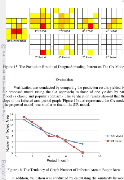
15 The Prediction Results of Dengue Spreading Pattern on CA model 27 16 The Tendency of Graph Number of Infected Area in Bogor Barat 27

LIST OF APPENDIX

A List the variables/attributes of DHF factors 30

B The survey forms 33

(15)

GLOSARY

Aedes aegypti is mosquito that could spread dengue fever, chikungunya, and yellow fever viruses, and other diseases

Emission probability is conditional distribution of observations given states Epidemic is the rapid spread of infectious disease to a large number of people in a

given population within a short period of time, usually two weeks or less Epidemiology is the science that studies the patterns, causes, and effects of health

and disease conditions in defined populations. It is the cornerstone of public health, and informs policy decisions and evidence-based practice by identifying risk factors for disease and targets for preventive healthcare. Ergodic HMM is one for wich underlying Marcov chain is ergodic, or at least is

irreducible and admits a unique stationary distribution.

Neighborhood is is a geographically localized community within a larger city, town, suburb or rural area

Spatiotemporal is the existing in both space and time.

(16)

(17)

1

INTRODUCTION

Background

Modeling aims to study and understand the phenomena by simplifying of a real problem. In epidemiology, system modeling approach is commonly used for viewing the epidemic process (Cuesta 2013). Most of the models for epidemics simulations are based on Ordinary Differential Equations (ODE) or statistical model (Pfeiffer 2008, White et al. 2007, Nishiura 2006). Moreover, visualization is required as the first step in an epidemiological analysis to understand the spatial characteristics of a dataset (Pfeiffer 2008). Pfeiffer (2008) also mentioned that visualization is needed for identifying the epidemiology of disease pattern in a given geographical area, predicting the spreading pattern of disease in the next period, and creating awareness for the target stakeholders based on the prediction results, hence helps clinical management of disease. Unfortunately, ODE or statistical models are unable to elaborate spatial patterns and interactions such as in the visualization and prediction of spreading disease (White et al. 2007).

In order to overcome these limitations, researchers used Celluar Automata (CA) models for involving time and space in epidemic process analysis (Santos et al. 2011). Some studies has been conducted such as developing a mathematical model of disease spread and its simulation using CA (White 2009), analyzing some scenarios of disease spread (Lopez et al. 2013), applying the CA approach to the Susceptible-Infective-Recovered (SIR) model of disease spread by considering birth and death factors and the changes of rules for each state in the dynamic CA (Athithan et al. 2014), and analyzing the complex spatiotemporal patterns observed in transmission of vector infectious disease (Santos et al. 2009).

Basically, CA is one of the dynamic system approaches that implementing discretization of time and space (White et al. 2007, Santos et al. 2011, Elsayed et al. 2013). CA consists of cells, called cellular space, a local connection of to other cells, and boundary conditions (White 2009). Each cell, representing a state, could change at every time-step using local transmission rules which would generate a new state based on the previous state of the cell and its neighborhood. Therefore, the concept of neighborhoods is very important. Santos et al. (2011) showed the effects of neighborhood structures on diseases spreading by using the Susceptible-Infected (SI) epidemics CA-model (Santos et al. 2011). Moreover, Hagoort et al. (2008) described the rule of neighborhood in determining the model interacts (Hagoort et al. 2008).

(18)

2

effectiveness of the proposed model, this approach was implemented to the Dengue Fever case.

The reason of using the Dengue Fever case is because it includes as one of the deadly and infectious pandemic diseases in Indonesia. This disease, also called Dengue Hemorrhagic Fever (DHF), is caused by the Dengue virus and is transmitted by the Aedes aegypti mosquito as a vector. Several studies related to the monitoring DHF in Indonesia have been conducted, such as the studies that aimed to see the trend of dengue outbreak in the future by Saragi (2011) and Octora (2010) (Saragi 2011, Octora 2010). Saragi (2011) used the Time Series method for showing the trend of dengue outbreak (Saragi 2011). The study predicted the number of dengue fever patients for next four years based on DHF patient data in the province of North Sumatra from 2005 to 2009. Octora (2010) compared the Autoregressive Integrated Moving Average (ARIMA) and the Winter approach to predict the number of DHF cases in the next six months (Octora 2010). This research used DHF cases data from Surabaya from January 2005 - June 2010. In this study, Octora (2010) applied four models of the Winter method and three models of the ARIMA method.

This paper explained how to develop a spreading pattern model of DHF on CA model that was used for visualizing and predicting spreading pattern of DHF. This study was especially focused on determining a probabilistic function using HMM with the dataset from a limited area such as West Bogor in the period of 2013. These dataset was used for defining the state criteria. Moreover, this study only considered an infective state which was dedicated particular attention to the spatial distribution of infected areas.The evaluation was conducted by comparing the results of the proposed model to that of one yielded by the SIR method, as a classical approach.

Problem Statement

As the problem definition above, the formulation of the problem in this study could be described as follows:

1. How to develop a visualization model of spreading pattern of the Dengue Fever.

2. How to predict the spreading process of Dengue Fever. 3. How to evaluate performance of our proposed model.

This research did not use real data cases of DHF for the following year because when data collecting was conducted, the availability of data had not been completed yet. Therefore, simulated data, as spreading initialization, was used for viewing and predicting the spread of DHF from the proposed model. The simulated data were generated randomly from John von Neumann-Random Generator based on CA rule. For evaluating the model, the proposed model was compared to the popular and accurate existing prediction mode such as SIR.

(19)

3 1. To develop a visualization model of spreading pattern of the DHF based on

CA approach supported by HMM 2. To predict the spread process of DHF.

3. To evaluate the performance of the model by comparing the results of the obtained model to that of one yielded by SIR method, as a classical approach.

Benefits

The contribution of this study is to provide information for researchers in epidemiology and government, especially for units under Departement of Public Health, in order to create a recommendation for controlling and preventing the spreading of Dengue disease.

Boundaries

This study only considered the dataset that contains of the DHF cases occurred in West Bogor in 2013. The spreading disease is commonly affected by some factors including birth, death, and density of mosquito, and population movement. In the case of DHF, the factors of birth and death could be ignored since the number of cases is quite small compare to the number of population. However, although there is only one occurrence of DHF, this occurrence should have to be handled. In addition, in the development of a model, the definition of Susceptible was changed from the number of populations to the number of infected regions. Therefore, it was assumed that the factor of population movement did not have a significant influence to the spreading disease of DHF. Thus, the factor of population movement could be ignored. The other factor that could be considered is the density of mosquito. However, in this research, those kinds of data could not be provided yet. Thus, by only considering the existing data cases for each period in every region, the HMM was chosen as a suitable

(20)

2

LITERATURE REVIEW

Epidemiology

Epidemiology is the field of study which is focused on exploring the causative factors of disease and the distribution of health in the certain region (Cuesta 2013). Cuesta (2013) stated that this study is very important since a plague could undermine human and cause the economic losses. Cuesta (2013) draw the elements of epidemiology as shown in Figure 1 as follow:

Figure 1 The triangle cart of the epidemiology elements (Cuesta 2013) Epidemic in a certain region is affected by the basics elements that related each others, such as pathogens from the susceptible population. In Figure 1 pathogens are represented by Agent. Pathogens would spread in a certain population. This spreading of disease is actually related to the population behavior in a certain evnvironment. Moreover, the environment is defined as an external condition that may cause the disease spread. Some environmental factors are geography, demography, climate, and social customs. The interaction among all elements, such as Agent, Population, and Environment in the range of period, describes a seasonal diseases.

Dengue Hemorrhagic Fever (DHF)

DHF is one of the deadly epidemics diseases that permanently exist in the certain region with the certain population (Cuesta 2013). DHF is caused by dengue virus transmitted to human by Aedes aegypti as a vector through his bite (Candra 2010). Based on Candra (2010) researches, the number of dengue cases has never decreased, even tends to increase, especially in the tropics or sub-tropics. DHF is able to infect any age, especially those who are less active.

Environment

Population Agent

(21)

5 SIR Model

The most common model used in the epidemiology fields where describes an infectious disease in a population is a SIR model, described as a state diagram in Figure 2 (Cuesta 2013) as follows:

Figure 2 SIR model (Cuesta 2013)

In his book, Cuesta (2013) described the SIR model as a state diagram that consists of three states including Susceptible (S), Infected (I), and Recovered (R). State S represents members of a population who are at risk of becoming infected. State S interacts with members of a population who are infected, I. There are two possibles conditions of an individu who is in state I. The fist condition is an individu would be still infected during the period of infection, indicated in Figure 2 by an arrow toward itself. The second condition is the individu become to be recovered, R.

The SIR model solves by mathematical approach using Ordinary Differential Equation(ODE). The ODE of SIR represented as follow:

dS

S I

dt     (1) dI

S I I

dt       (2) dR

I

dt   (3)

where S = number of susceptible, I = number of infectious, and R = number of recovered. Case represents the transmission probability of the disease while represents the period of infection.

Model Cellular Automata (CA)

(22)

6

CA model is a model that represents data objects observed as grid of cells in which in a neighborhood, each cells influence each other (Maeda 2006). In this study, Maeda (2006) defined that in the next period, a cell (initial state) which interacts with other one in a neighborhood would be changed into a new state (next state). The way of how a neighborhood affects a cell (from initial state to next period) is called as CA rule. The two dimensional CA is defined as a model on a discrete system dynamic with some objects regularly spread in the two dimensional space or coordinate space (Figure 3) in which each cells is assigned with an initial state (White 2009). In the case of 2-dimensional CA, there are two basic forms of neighborhood including Von Neumann–neighborhood and Moore– neighborhood. Von Neumann–neighborhood with r = 1, has size of 5, consists of a center cells and 4 neighborhood cells, upside, down side, left side, and right side (Figure 4 (a)). Moore–neighborhood with r = 1, has a size of 9 consists of a center cell and 8 neighborhood cells close each other (Figure 4 (b)).

Figure 3 Two-dimensional cellular space (Elsayed et al. 2013)

Figure 4 (a) Von Neumann-neighborhood (b) Moore-neighborhood (Elsayed et al. 2013)

The extention of a neighborhood is determined by parameter of radius (r), the distance of a cell to the cell farthest from the neighbors that may affect the cells in a state change. Size of Moore-neighborhood could be calculated with the following equation (Maeda 2006):





2

1

n r (4)

(23)

7 Composing Neighborhoods

One of the important steps in modeling of CA is how to determine neighborhood cells spatially. There are three techniques related to spatial neighborhood relationship, including topological, distance, and direction relation which may be combined by logical operators to express a more complex neighbourhood relation (Ester et al. 2001). In spatial problem, the most important object is point. The other objects such as lines, polygons or polyhedrons are represented by a set of points.

Topological relations, the first technique in determining spatial neighborhood relationship, are determined by considering the boundaries, interiors and complements of the two related objects. These relations remain unchanged when transformations are applied. There are some types of transformations such as continuous, one-one, onto and whose inverse is continuous. The relations are: A disjoint B, A meets B, A overlaps B, A equals B, A covers B, A covered-by B, A contains B, A inside B.

The second technique is Distance relations. This technique used the arithmetic comparison operators in order to compare the distance of two objects with a given constant. In the case of the distance based technique, a distance relationship is determined by calculating the distance between two objects, A and B. The third technique is the direction relations. Figure 5 illustrates the definition of some direction relations using 2D polygons. Obviously, the directions are not specifically defined but there is always a smallest direction relation for two objects A and B, called the exact direction relation of A and B, which is uniquely determined.

Figure 5 The illustration of determining neighborhood technique (Ester et al. 2001)

Hidden Markov Model

(24)

8

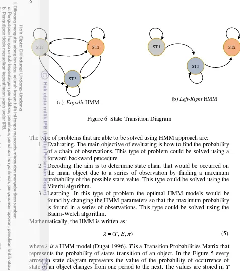
(a) Ergodic HMM (b) Left-Right HMM

Figure 6 State Transition Diagram

The type of problems that are able to be solved using HMM approach are:

1. Evaluating. The main objective of evaluating is how to find the probability of a chain of observations. This type of problem could be solved using a forward-backward procedure.

2. Decoding.The aim is to determine state chain that would be occurred on the main object due to a series of observation by finding a maximum probability of the possible state value. This type could be solved using the Viterbi algorithm.

3. Learning. In this type of problem the optimal HMM models would be found by changing the HMM parameters so that the maximum probability is found in a series of observations. This type could be solved using the Baum-Welch algorithm.

Mathematically, the HMM is written as: ( , , )T E

  (5)

whereλ is a HMM model (Dugat 1996). T is a Transition Probabilities Matrix that represents the probability of states transition of an object. In the Figure 5 every arrow in state diagram represents the value of the probability of occurrence of state of an object changes from one period to the next. The values are stored in T

as shown in Table 1.

Table 1. The Transition Probability values nth Period

ST1 ST2 ST3 Σ

(n-1)th Period

ST1 P(a|a) P(b|a) P(c|a) 1

ST2 P(a|b) P(b|b) P(c|b) 1

ST3 P(a|c) P(b|c) P(c|c) 1

ST1 ST2

ST3

ST1 ST2

(25)

9 E is an Emission Probabilities Matrix that represents the probabilities of an object to be in a certain state which is affected by state conditions of the surrounding of the other observed object.The values are stored in Eas shown in Table 2. Prior Matrix, π, is a probabilities matrix of an object on the beginning of the sequence of events was in a certain state. The values are stored in πas shown in Table 3.

Table 2. The Emission Probability values An Observed Object

(Xi)

X1 X2

a1 b1 a2 b2

ST1 P(a1|ST1) P(b1|ST1) P(a2|ST1) P(b2|ST1)

Σ 1 1 1 1

Table 3. The Prior Probability values ST1 P(ST1) ST2 P(ST2)

ST3 P(ST3)

Σ 1

The probability of an objek C be a certain state condition at the time i, denoted byP(C |_i X_i), which is affected by the state condition of the observed surrounding objects X is able to be calculated using Bayes theory

( | C ). (C ) (C | )

( )

i i i

i i

i

P X P

P X

P X

 (6)

where (C )P _i is a transition probability value of state changes of an object C from time at i-1 to i, and P X( _i| C )_i is an emission probability value of changing states of an object X with the certain state condition of C at that time. Generally probability of an object C be a certain state condition at the time n, denoted by

1 2 1 2

( , ,..., _n| , ,..., _n)

P C C C X X X , for a moving time from i = 1 to i = n could be written as follows:

1 2 1 2 1

1 1

( , ,..., | , ,..., ) ( | ). ( | )

n n

n n i i i i

i i

P C C C X X X P X C P C C_

 





(7)

where P C C( _i| _i_₁) is a transition probability value of state changes of an object C

(26)

3

METHODOLOGY

Research Framework

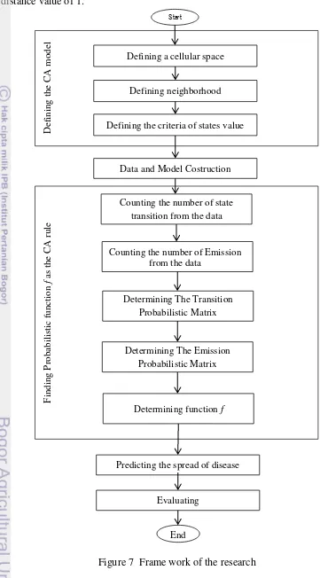
The objective of this research is to develop a model of disease spread using CA method. The contribution of this research is how to define parameters and rule function used in simulation development. Several stages were done to achieve the research objective, including: defining the CA model, collecting datasets and constructing the model, finding a probabilistic function as a CA rule, predicting the spread of disease using the proposed model, and evaluating the model. These analysis results would be the basic information for preventing of disease.

The main problem of this research is how to find a function that represents a proper CA rule, and the HMM was chosen as a method for determining a function that represents CA rule. Several steps on HMM were done to find the function including: counting the number of state transition, counting the number of emission, determining the Transition Probabilistic Matrix, and determining the Emission Probabilistic Matrix. Figure 6 shows all the stages of this study.

Defining a Spreading Pattern Model Based on CA Model

There are four steps for defining the CA model, such as: defining a cellular space, defining neighborhood used in a cellular space, defining the criteria of the possible state values, and determining some probability values of function f that represent the CA rule. Function f is required to obtain a spreading pattern of disease on CA model.

Defining a Cellular Space and Neighborhood

First steps, a map of regions were transformed into a rectangular polygon

Ci. Next, the polygons were composed in the cellular space as the same size cells.

Each cell defines ununiformed objects and describes the number of disease cases that occurred in the region. The index i of cell Ci stated the cell in the cellular

space. Each cell represents a region according to id of cell. A region position in a cellular space was determined using grid region rule based on distance approach (Figure 5). This approach was conducted by calculating distance to the surrounding region. The shortest distance was stated as Von Neumann neighborhood. The calculation of distance was conducted using Manhattan distance formula (Bajracharya and Duboz 2013) as follows:





2 1 1 2 ( , ) i i i i a b dist T T

n









(8)

where T1 and T2 are two regions in which the distance between them were

calculated using the equation 8, in which a represented the position of T1 and b

represented the position of T2. The calculation results of equation 8 were changed

(27)

11 value of 0. Moreover, two regions that have one region between them would have distance value of 1.

Figure 7 Frame work of the research

Def

in

ing

t

he

CA

m

od

el

Findi

ng Pro

bab

il

is

ti

c

fun

ct

ion

f

a

s t

h

e CA

r

u

le

Start

Counting the number of Emission from the data

Counting the number of state transition from the data Data and Model Costruction

Defining a cellular space

Defining neighborhood

Defining the criteria of states value

Determining The Transition Probabilistic Matrix

Evaluating

End

Predicting the spread of disease Determining The Emission

Probabilistic Matrix

(28)

12

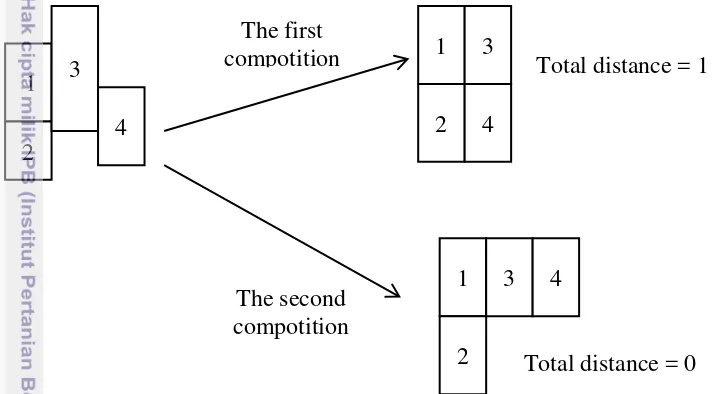
This research also defined a rule in which if there are two regions or more having direct boundary with one other region, then the total distance of all possible neighborhood composition would be counted. A neighborhood composition with the most minimum total distance would be chosen as region position composition in a cellular space. Figure 8 shows the example in which there are two possibilities in composing neighborhood. The first composition has total distance of 1, while the second composition has total distance of 0. In this case, the second composition was chosen since it had the most minimum total distance.

Figure 8 The possibility of a composing neighborhood

The number of cell in the cellular spaces actually has not always to be the same as the number of the observed regions. For instance, we are able to define 20 or 25 cellular spaces for the 16 observed regions by adding the definition of boundary condition for the regions which are not included into the 16 observed regions (White et al. 2007). Boundary condition is a cell condition whereas an observed cell does not have a complete number of neighborhoods since its position is in the corner or in the boundary side of cellular space. In the proposed model, a cell has incomplete neighborhood if i 4 0 or i 1 0 or i 1 16 or i 4 16. In this study, for the proposed model, we assumed null boundary conditions. Defining a cellular space was done by calculating the number of direct neighborhood of each region to compose regions in a cellular space.

Defining a Set of States

The research that related to the state changes of a cell in two-dimensional has performed by Djatna and Morimoto (2008). In this research, the concept of state change was used for selecting features. The state change was calculated based on the change of shape of the geometry which represented the affecting results of two dimensional rules which is applied to the pair of attributes (Djatna and Morimoto 2008). In the proposed model, the concept of state change was applied to visualize the spreading pattern of disease. We defined a state changes based on data content on location. First, we defined the categories value in a

1 2

3 4

1

2 3

4

1

2

3 4

Total distance = 1 The first

compotition

The second compotition

(29)

13 number of categories, and set the color for each category. Next, the state changes were seen as cell color changes in a cellular space.

Data and Model Construction Collecting the Dataset

In this research, a CA model applied to DHF cases. Before conducting a data colection, we studied data characteristics related to DHF. The spread of dengue fever disease is influenced by several factors including condition of the environment, behavior of population and agent of disease vectors (in this case is the mosquito Aedes aegypti). Based on the literature study, generally, we noticed some variables/attributes which were important to be considered as causative factors of DHF. We listed the variables/attributes in Appendix A.

We decided to use dataset collected from Dinas Kesehatan Kota Bogor (DKK-Bogor). The data were collected using an interview technique. We did an interview with the DKK-Bogor Data Officer on July 16, 2014. The observation process of spreading disease of DHF in Dinas Kesehatan tingkat Kota, in Bogor was conducted by collecting reports from each Puskesmas in Bogor city. This process was conducted until the smallest government entity, called Kelurahan. The interview result was shown in Appendix B. In collecting the datasets, we did some steps as follows: identify of geographical study area, conducting field study for data collection, deciding sample used in this research, and determining the source of the data. We also decided to focus on the West Bogor which was divided into 16 regions.

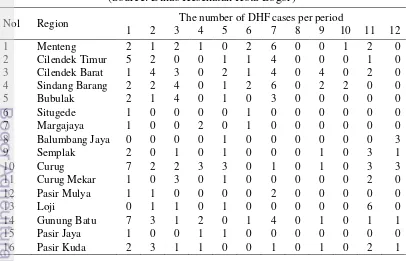
Table 4 Number of Dengue cases in West Bogor in 2013 (Source: Dinas Kesehatan Kota Bogor)

Nol Region The number of DHF cases per period

1 2 3 4 5 6 7 8 9 10 11 12

(30)

14

Data attributes used in this research are: “name of a region” and “number

[image:30.595.120.399.142.405.2]

of Dengue cases on 12 period”. In this research, we used the dataset that contains of the occurrence of DHF cases in West Bogor in 2013 shown in Table 4.

Figure 9 The map of regions in West Bogor

A Cellular Space Construction

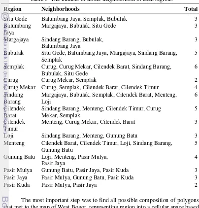
In this research, 16 cells in two-dimensional cellular space (Table 5) were defined representing 16 regions in West Bogor (Figure 9). This research used West Bogor that consisted of 16 regions. The total number of direct neighborhoods of 16 regions was listed in Table 4. Next, the map was transformed into 4X4 rectangular polygons as shown in Figure 10. The polygons should have the same size as cells in the cellular space. Each cell defines ununiformed objects and describes the number of dengue cases that occurred in the region.

[image:30.595.230.358.564.696.2]

(31)

[image:31.595.106.510.177.599.2]

15 The cellular space is defined as a two-dimensional space in which each cell represents a region with some Dengue cases in each period. The total region in West Bogor is 16 regions. Thus, we defined 16 cells. Each cell contained some un-uniformed objects that described some Dengue cases that occurred in a region for the certain period.

Table 5 The number of direct neighborhood of each regions

Region Neighborhoods Total

Situ Gede Balumbang Jaya, Semplak, Bubulak 3

Balumbang Jaya

Margajaya, Bubulak, Situ Gede 3

Margajaya Sindang Barang, Bubulak, Balumbang Jaya

3 Bubulak Situ Gede, Balumbang Jaya, Margajaya, Sindang Barang,

Semplak

5 Semplak Curug, Curug Mekar, Cilendek Barat, Sindang Barang,

Bubulak, Situ Gede

6

Curug Curug Mekar, Semplak 2

Curug Mekar Curug, Semplak, Cilendek Barat, Cilendek Timur 4 Sindang

Barang

Margajaya, Bubulak, Semplak, Cilendek Barat, Menteng, Loji

6 Cilendek

Barat

Sindang Barang, Menteng, Cilendek Timur, Curug Mekar, Semplak

5 Cilendek

Timur

Menteng, Curug Mekar, Cilendek Barat 3

Loji Sindang Barang, Menteng, Gunung Batu 3

Menteng Cilendek Barat, Cilendek Timur, Loji, Sindang Barang, Gunung Batu

5 Gunung Batu Loji, Menteng, Pasir Mulya,

Pasir Jaya

4

Pasir Mulya Gunung Batu, Pasir Jaya, Pasir Kuda 3

Pasir Jaya Pasir Mulya, Gunung Batu, Pasir Kuda 3

Pasir Kuda Pasir Mulya, Pasir Jaya 2

The most important step was to find all possible composition of polygons that met to the map of West Bogor, representing region into a cellular space based on the data on Table 4. Next, the total distances of the possibility compositions were calculated using equation (8) for obtaining the minimum total distance.

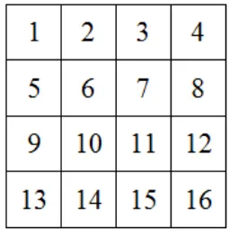
In data construction, each cell was defined as a one-dimensional array variableX 



X_i/i1, 2,..,16



. Variable Xi represented a cell as shown in Figure

10.

Neighborhood

(32)

16

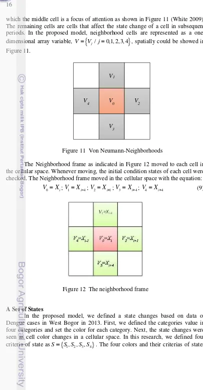
[image:32.595.73.478.54.831.2]

which the middle cell is a focus of attention as shown in Figure 11 (White 2009). The remaining cells are cells that affect the state change of a cell in subsequent periods. In the proposed model, neighborhood cells are represented as a one-dimensional array variable, V 



V_j/ j0,1, 2,3, 4



, spatially could be showed in Figure 11.

Figure 11 Von Neumann-Neighborhoods

The Neighborhood frame as indicated in Figure 12 moved to each cell in the cellular space. Whenever moving, the initial condition states of each cell were checked. The Neighborhood frame moved in the cellular space with the equation:

0 i

V  X ; V₁X_i_₄; V₂ X_i_₁; V₃  X_i_₄; V₄ X_i_₄ (9)

Figure 12 The neighborhood frame

A Set of States

In the proposed model, we defined a state changes based on data of Dengue cases in West Bogor in 2013. First, we defined the categories value in four categories and set the color for each category. Next, the state changes were seen as cell color changes in a cellular space. In this research, we defined four criteria of state asS 



S S S S₁, ₂, ₃, ₄



. The four colors and their criterias of states

V1

V₀

V₃

V₄ V₂

(33)

17 are shown in Table 6. In data construction, states value was represented by an array, with the array variable ofS 



S S S S₁, ₂, ₃, ₄



.

Table 6 State definition of infected area

State State definition State colour

S1 : all peoples have been recovered, or no one was infected S2 : 1-2 peoples were infected

S3 : 3-5 peoples were infected S4 : > five peoples were infected

The construction for another data was shown in the Table 7. In this research, Excel spreadsheets as a tool was used to build a simulation model to find a probabilistic function and a spreading pattern. Moreover, a Scipy module in Python 3.4 (https://github.com/hmcuesta/PDA_Book/tree/master/Chapter9) as tool was used for evaluating the proposed model.

Finding a Probabilistic Function

The next step is how to determine a function f that represents the CA rule based on parameters defined. In detail, our method for defining the CA model was described as follows. Firstly, from the dataset that consist of 16 regions, we defined the two-dimensional space and put each region into a one cell and set an index for each cell, then we defined an array variable to represent the 16 cells in which each cell has an index. Next, we put the number of data cases for each region (number of infected) into an array variable in which data in one period were stored into an array variable, running as time-step. Finally, with a set of states criterias, we replaced the data cases with the data states.

The main problem of this research is how to find the function that

represents a proper CA’s rule. Many methods to find function f as rule of CA model have been conducted, and in this research we used HMM, a method that has not been used by researchers yet. In HMM the state chages described as the state transition diagram. By ignoring the death factor and the birth factor, and by assuming that the probability of an infected cell is affected by surrounding cells that are considered an effective influence, then the HMM approach was suitable to be used to determine a probabilistic function f.

The CA characteristic was represented as a Markov process (Knutson 2011). Since the dataset was able to be classified as a time series dataset, it was proper to use a probabilistic function that could be found using HMM. HMM is a probabilistic model that is suitable for solving the problem related to the data sequential-temporal (Peng et al. 2011). In the proposed CA model, the state change of a cell to another state could be described as a State Transition Diagram (Figure 10). The State Transition Diagram was able to express in HMM model as

(34)

18

Table 7 List of the data construction

per Variable of period

SCij Two-dimensional array variable for the number of state change of V0

from Si to Sj in a period to the next period.

i = 1..4; j = 1..4

SSi One-dimensional array variable for the sum of state change of V0

from Si.

i = 1..4

Tij Two-dimensional array variable for the transition probability matrix

of V0.

ij ij i SC T SS

 ; i = 1..4; j = 1..4

V1ij Two-dimensional array variable for the number of V0 in Si state

condition when V1 in Sj state condition. i = 1..4; j = 1..4

SV1i One-dimensional array variable for the sum of V0 in Si state condition

when V1 in any state. i = 1..4

E1ij Two-dimensional array variable for the emission probability matrix

of V0 affected by V1.

1 1 1 ij ij i V E SV

 ; i = 1..4

(35)

19

Figure 13 State Transition Diagram of proposed model Table 8. Transition Probabilities Matrix

Period n-1 Period n

S1 S2 S3 S4 Σ

S1 P(S1|S1) P(S1|S2) P(S1|S3) P(S1|S4) 1

S2 P(S2|S1) P(S2|S2) P(S2|S3) P(S2|S4) 1

S3 P(S3|S1) P(S3|S2) P(S3|S3) P(S3|S4) 1

S4 P(S4|S1) P(S4|S2) P(S4|S3) P(S4|S4) 1

Based on the criteria of state shown in Table 5, we used Ergodic HMM model (Figure 13) that mathematically is written in equation (5) to get a probabilistic function (Terry 2007). Each arrow in the state diagram represented a probability value of an object to change the value of state from one period to the next one. The values were stored in T as shown in Table 8.

The Emission Probabilities were stored in E as shown in Table 9. In this study, we assumed that the initial state of a cell at the beginning of the period had the same probability of possible states values. Thus, the prior probabilities were ignored.

Table 9. Emission Probabilities Matrix Main Object

(C)

Observed Object (Vi)

S1 S2 S3 S4

Σ 1 1 1 1

To find the values of T and E from the data, firstly, we counted the number of state changes from S1-S1, S1-S2, …, S4-S3, S4-S4 to determine matrix of

transition probabilities 1 0 0 ( n| n )

(36)

20

Table 10 List of a state change No. of list The state change

1. S1 to S1 from period to the next period 2. S1 to S2 from period to the next period 3. S1 to S3 from period to the next period 4. S1 to S4 from period to the next period 5 S2 to S1 from period to the next period 6. S2 to S2 from period to the next period 7. S2 to S3 from period to the next period 8. S2 to S4 from period to the next period 9. S3 to S1 from period to the next period 10. S3 to S2 from period to the next period 11. S3 to S3 from period to the next period 12. S3 to S4 from period to the next period 13. S4 to S1 from period to the next period 14. S4 to S2 from period to the next period 15. S4 to S3 from period to the next period 16. S4 to S4 from period to the next period

The values of the calculation results of list in Table 10 were stored in a table in which its format could be shown in Appendix C. These data were inputted to the equation (10) to yield the probability values of the state transition which is stored into a matrix as shown in Table 8. In HMM, this matrix is set as the Transition Probabilities Matrix (T).

T = ( | ) ij

i

S P Si Sj

S





(10)

Next, the CA case could be associated as the case that has a hidden state. The changing of state V0 in the next period is affected by the state of

neighborhood cells V1, V2, V3, V4. Thus, the emission probability P V( i |V0 ) could be calculated. In the domain of HMM, the proposed model based CA is classified as Decoding problem in HMM. V0 is an object in which its state change will be

predicted in the next period observed. The neighborhood cells V1, V2, V3, V4, are

objects in which each of them could have state S1, S2, S3 or S4 in the current

period and affect the change of state of V0 in the next period.

In the proposed model, V0 represented region defined as a focused cell

shown in Figure 9. This focused cell moved from the first index to the 16th index and contained data cases for the period of 1 to 12. From these data cases and using Von Neumann neighborhood, we counted the number of state change of V0

from states condition when the four neighborhoods V1, V2, V3, V4 were in certain

(37)

21

E = ( | ₀ S ) j Vi

i j

Vi

S P V V

S

 



(11)

Eventually, the total value of the probability of the transition of V0 could

be calculated by Bayesian formula shown in equation (7) for each possible states of V0.

Prediction of Pattern of the Disease Spread

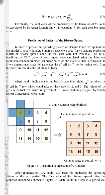
In order to predict the spreading pattern of Dengue Fever, we applied the CA model to a new dataset. Simulated data were used for visualizing prediction results of disease spread since the real data were not available. The initial conditions of DHF cases of each region were simulated using the John von Neumann-Random Number Generator based on the CA rule, that is equivalent to a two-dimensional space for generates the jth cell in ith-row by taking cells from the previous row (Gentle 2003) as follows:





( ) ( 1) ( 1) ( 1) ( 1) ( 1)

1 1 1 mod 4

i i i i i i

j j j j j j

x



x

 

x

 

x

 

x x

  (12) where mod 4 indicates the number of states that might,

x

( )_ji describes the [image:37.595.89.508.36.807.2]

jth cell in ith-row which could take on the value 0,1,2, and 3. The values of the cells in the first row, which range from 0 to 3, were randomly assigned by Simple Linear Congruential Generators.

Figure 14 Illustration of algorithm of CA model

After initialization, CA model was used for predicting the spreading pattern of the next period. The illustration of the diseases spread using the proposed model was shown in Figure 14. State value in a cell in a period will

Von Neumann Neighborhood

Cellular space at period t = i

(38)

22

change on the next period by the function f that worked over the frame-neighborhoods moves. Stopping condition was reached when state value would not be changed again for the next period.

For instance, at a period of ti, started with a cell C1 , a cell with index =

1), using the Von Neumann Neighborhood frame, function of f as CA rule was applied to affect C1 by considering the conditions of C2 and C5, two neighborhood

cells of C1. f yield the most possible state condition of C1 at the next period of 1

t i . Next, neighborhood frame moved to C2 in which the condition of C1, C3

and C6 as its neighborhood cells would affect the condition of C2 in the next

period. This procedure was repeated from the cell of C1 to the cell of C16. Thus,

after t = i+1, the state of all cells in the cellular space had been changed. These steps were repeated again for the period of t = t+2 and so on. The change of all cells from ti, t  i 1,t i 2,…, tn yielded the patterns of disease spread. This process was stopped when the state value of all cells remained the same for the next period.

Verification and Validation

We evaluated the proposed models by conducting verification and validation. Model verification aims to ensure that the CA model has been implemented correctly. Moreover, the purpose of validation is to determine whether the theory and assumptions underlying the preparation of this model are correct (Sargent 2007). The SIR-model is a simple mathematical model based on ODE that has been proven to be an acceptable model in epidemic fields (Bootsma and Ferguson 2007).

We verified the model by comparing the tendency of graphs yielded by the proposed model, and the trend graphs yielded by the SIR model. Sequentially we validated the model by measuring the proximity of the simulation results of the proposed model and those of the SIR-model using a correlation coefficient measure to compute similarity (Cha 2007):

1

(x )(y ) ( , ) ( 1) n i i i X Y x y

Corr X Y

n  

    



(13)

where x_i and x are defined as time-series data and the average generated by the proposed model, respectively. In the same definition, y_i and y are defined for the SIR model. i represents periods from i = 1, 2, .., n. In this study, X represents the vector of number of infected area during a one period, yielded by the CA model, while Y represents the vector of number of infected area during a one period, yielded by the SIR model. _X and _Y represent standard deviations of variable X

(39)

4

RESULTS AND DISCUSSION

The Spreading Pattern Model based on CA The Cellular Space

The composition of regions in cellular space of 4x4 cells (Figure10) that optimal was shown in Table 11. The index i for cell Ci (Figure 10) state as a cell

in the cellular space with each cell represents a region according to id of cell listed in Table 11; for instance, the first cell with index = 1 in Figure 10 represents a region of Situ Gede (a region with id 1 in Table 11).

Table 11 The cells representing the region

I Region (Ci)

1 Situ Gede

2 Bubulak

3 Curug

4 Curug Mekar

5 Balumbang Jaya

6 Sindang Barang

7 Semplak

8 Cilendek Timur

9 Margajaya

10 Menteng

11 Cilendek Barat

12 Pasir Jaya

13 Gunung Batu

14 Loji

15 Pasir Mulya

16 Pasir Kuda

The Probabilistic Function as Rule on CA Model

Transition Probabilities Matrix

The number of state changes calculated by using data cases of DHF in West Bogor, in 2013 (Table 9). The calculation results could be shown in Table 12. The values of a transition probabilities matrix 1

0 0 ( n | n )

P V V  were calculated from data on Table 12 and represented as the probabilities values as follows:

0.60 0.32 0.06 0.01

0.54 0.30 0.13 0.03

0.59 0.24 0.18 0.00

0.60 0.20 0.20 0.00 1

( | )

0 0

n n P V V

     __ _       (14)

In this matrix, we saw that the change from state S4 to S1 has the highest

(40)

24

the condition of a cell was in the state of S4, the state tent to change to the better condition because the probability of the cell’s state to keep its state was very small

[image:40.595.73.489.156.803.2]

or never occurred. It means that there were always the preventive actions to stop the spreading of Dengue Fever diseases in this area.

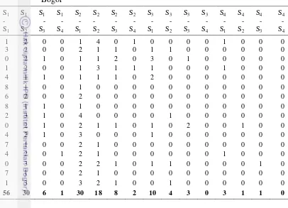
Table 12. The number of state changes based on the data cases of DHF in West Bogor S1 - S1 S1 - S2 S1 - S3 S1 - S4 S2 - S1 S2 - S2 S2 - S3 S2 - S4 S3 - S1 S3 - S2 S3 - S3 S3 - S4 S4 - S1 S4 - S2 S4 - S3 S4 - S4

1 2 0 0 1 4 0 1 0 0 0 0 1 0 0 0

3 2 0 0 2 1 1 0 1 1 0 0 0 0 0 0

0 2 1 0 1 1 2 0 3 0 1 0 0 0 0 0

1 2 0 0 1 3 1 1 1 0 0 0 1 0 0 0

4 1 1 0 1 1 1 0 2 0 0 0 0 0 0 0

8 1 0 0 1 0 0 0 0 0 0 0 0 0 0 0

6 2 0 0 2 0 0 0 0 0 0 0 0 0 0 0

8 1 1 0 1 0 0 0 0 0 0 0 0 0 0 0

2 3 1 0 4 0 0 0 0 1 0 0 0 0 0 0

0 2 1 0 2 1 1 0 1 0 2 0 0 1 0 0

4 2 1 0 3 0 0 0 1 0 0 0 0 0 0 0

7 1 0 0 2 1 0 0 0 0 0 0 0 0 0 0

4 2 0 1 2 1 0 0 0 0 0 0 1 0 0 0

0 3 0 0 2 2 1 0 1 1 0 0 0 0 1 0

7 1 0 0 2 1 0 0 0 0 0 0 0 0 0 0

1 3 0 0 3 2 1 0 0 1 0 0 0 0 0 0

56 30 6 1 30 18 8 2 10 4 3 0 3 1 1 0

Emission Probabilities Matrix

The emission probabilities could be obtained by conducting the similar procedure for calculating the transition probabilities matrix. By using data cases in West Bogor, in 2013 and using the Von Neumann-neighborhood, we counted the number of state change of an area affected by surrounding area. The results were shown in Table 13. There are four observed objects V1, V2, V3, V4. Each object

could be in state S1, S2, S3, or S4. From the data in Table 13 and by using formula on the equation (10) the Emission Probabilities values were calculated. The calculation also yielded four Emission Probability matrixes (E).

Table 13 The counter result of states changes affected by neighborhood

V1 V2 V3 V4

V0 S1 S2 S3 S4 S1 S2 S3 S4 S1 S2 S3 S4 S1 S2 S3 S4

[image:40.595.81.487.179.472.2]

(41)

25 In this research, E is a matrix for representing the state change probabilities of a certain area affected by its neighborhood. There are four matrices E as sequently Eq. 15 up to Eq. 18 as follows.

0.6579 0.2500 0.0789 0.0132

0.4423 0.4038 0.1346 0.0192

0.5833 0.2500 0.1667 0.0000

0.0000 0.5000 0.2500 0.25 ( | )

1

00 0

P V V

             (15)

Equation (15) described the probability of a state change of cell V1 on the

next period that is affected by the state change of cell V0. It was shown that the

probability of V1’s state change to S4 was very small or never occurred, while V0

was in S3. Moreover, this matrix also showed that the change from the state of

area V1 to S1, while V0 was in S4 was never occurred.

0.6538 0.2692 0.0769 0.0000

0.4255 0.4255 0.1277 0.0213

0.4667 0.2667 0.2000 0.0667

0.2500 0.5000 0.2500 0.00 ( | )

2

00 0

P V V

             (16)

From the equation (16), we saw that the state change of V2 to S4, affected

by V0, would never occur while the state of V0 is in the condition of S1 or S4. 0.6250 0.2875 0.0875 0.0000

0.4222 0.4667 0.0667 0.0444

0.3750 0.4375 0.1250 0.0625

0.3333 0.3333 0.0000 0.33 ( | )

3

33 0

P V V

             (17)

next period that was affected by the state condition of V0. 0.6456 0.2532 0.0886 0.0127

0.4468 0.4255 0.0851 0.0426

0.3750 0.3750 0.1875 0.0625

0.0000 0.5000 0.5000 0.00 ( | )

4

00 0

P V V

      _ _     (18)

next period that was affected by the V0 state condition. From the four matrices

above, it was concluded that the extreme change conditions of the neighborhoods to S4, affected by the focus area, were very rare.

The probabilistic function f was found by using HMM approach.

Mathematically, it’s could be found by Bayes theorem, including the emission

probabilities formula and the transition probabilities formula. As shown in equation (19).

4

4 ₁

( | S ). ( S | )

max ₀ ₀ ₀

i 1 1

n n n

f P V V P V V

j i i

j    _           _  _ (19) where ₀n

V represents state value of cell V0 in n-th period, and ( | 0 1)

n n

o i

(42)

26

choose the maximum value of the probability of the state change. It means that the change of a state in the cell of V0 in the next period depends on the maximum

probability value obtained from equations (20-23). These probabilities consist of four possibility values that are defined as follows.

4

1

( S | , , , ) ( | S ). ( S | )

0 1 1 2 3 4 0 1 0 1 0

1

n n n n

P V V V V V P V V P V V

i i        (20) 4 ₁

( S | , , , ) ( | S ). ( S | )

0 2 1 2 3 4 0 2 0 2 0

1

n n n n

P V V V V V P V V P V V i i        (21) 4 ₁

( S | , , , ) ( | S ). ( S | )

0 3 1 2 3 4 0 3 0 3 0

1

n n n n

P V V V V V P V V P V V i i        (22) 4 ₁

( S | , , , ) ( | S ). ( S | )

0 4 1 2 3 4 0 4 0 4 0

1

n n n n

P V V V V V P V V P V V i i        (23)

The values of ( | 0 S )1

n i

P V V  _; P V V( |_i ₀nS )₂ _; P V V( |_i ₀nS )₃ _; P V V( |i ₀nS )₄ were obtained from The Emission Probabilities Matrix using the equations (15-18). Moreover, the values of

1

0 1 0

( n S | n )

P V  V  _; 1

0 2 0 ( n S | n )

P V  V  _; P V( ₀nS |₃ V₀n1)_; 1

0 4 0

( n S | n )

P V  V  _{were obtained from}_T_{, where}_T₌ 1 0 0 ( n| n )

P V V 

was obtained from Transition Probability Matrix (Eq. 14).

The output of the f (eq. 19) is a maximum probability value that related to the state where a cell would be changed. At this point so far, the proprosed model has already completely defined. Thus, the first objective was successfully achieved.

Prediction Spreading Process of DHF using The Proposed Model The spreading pattern of the prediction model were represented by the probabilistic function that represents the CA rule. An example of the simulation results was shown in Figure 15. The pattern was able to obtained using equation (19). The inputs to this equation were the Transition Probability Matrix (Eq. 14), the Emissions Probability Matrix (Eq. 15-18), and the randomized data initialization that was obtained by equation (12). The visualization of the obtained pattern results indicated that