Forecasting spare parts demand: a case study at an indonesian heavy equipment company

(1)

FORECASTING SPARE PARTS DEMAND: A CASE STUDY

AT AN INDONESIAN HEAVY EQUIPMENT COMPANY

RYAN PASCA AULIA

DEPARTMENT OF STATISTICS

FACULTY OF MATHEMATICS AND NATURAL SCIENCES

BOGOR AGRICULTURAL UNIVERSITY

(2)

(3)

PERNYATAAN MENGENAI SKRIPSI DAN

SUMBER INFORMASI SERTA PELIMPAHAN HAK CIPTA

Dengan ini saya menyatakan bahwa skripsi berjudul Forecasting Spare Parts Demand: A Case Study at an Indonesian Heavy Equipment Company adalah benar karya saya dengan arahan dari komisi pembimbing dan belum diajukan dalam bentuk apa pun kepada perguruan tinggi mana pun. Sumber informasi yang berasal atau dikutip dari karya yang diterbitkan maupun tidak diterbitkan dari penulis lain telah disebutkan dalam teks dan dicantumkan dalam Daftar Pustaka di bagian akhir skripsi ini.

Dengan ini saya melimpahkan hak cipta dari karya tulis saya kepada Institut Pertanian Bogor.

(4)

ABSTRACT

RYAN PASCA AULIA. Forecasting Spare Parts Demand: A Case Study at an Indonesian Heavy Equipment Company. Advised by FARIT MOCHAMAD AFENDI and YENNI ANGRAINI.

Forecasting spare parts demand is a common issue dealt by inventory managers at maintenance service organization. The large number of items held in stocks and the random demand occurrences make most of the difficulties. An Indonesian heavy equipment company targets to advance its forecast accuracy. Accordingly, this study has two main goals. Firstly, all Stock Keeping Units (SKUs) are classified based on their demand patterns, utilizing their average inter-demand interval (ADI) and squared coefficient of variation (CV2) of demand sizes as the classifiers. After that, four simple forecasting methods are applied to each demand class and the best forecasting method in term of its forecast errors is chosen. Evaluation of forecast accuracy is made by means of the Mean Absolute Scaled Error (MASE), MAD-to-Mean ratio, and Percentage Best (PBt). The forecasting competition results show the dominance of Syntetos-Boylan Approximation for erratic, smooth, and intermittent demand, and Simple Moving Average for lumpy demand.

(5)

Scientific Paper

to complete the requirement for graduation of Bachelor Degree in Statistics

at

Department of Statistics

FORECASTING SPARE PARTS DEMAND: A CASE STUDY

AT AN INDONESIAN HEAVY EQUIPMENT COMPANY

RYAN PASCA AULIA

DEPARTMENT OF STATISTICS

FACULTY OF MATHEMATICS AND NATURAL SCIENCES

BOGOR AGRICULTURAL UNIVERSITY

(6)

(7)

Title : Forecasting Spare Parts Demand (A Case Study at an Indonesian Heavy Equipment Company)

Name : Ryan Pasca Aulia NIM : G14100017

Approved by

Dr Farit M Afendi, MSi Advisor I

Yenni Angraini, MSi Advisor II

Acknowledged by

Dr Anang Kurnia, MSi Head of Department

(8)

ACKNOWLEDGEMENTS

Great thanks to God Almighty for the strength, willingness and opportunity given to me so that I might be able to complete this paper which is entitled Forecasting Spare Parts Demand: A Case Study at an Indonesian Heavy Equipment Company. This study is motivated by my literature research during the internship program held by the Department of Statistics, Bogor Agricultural University.

I realize that this research could not happen without the support of many people. Therefore, I would like to express my gratitude to my advisors, Dr Farit M Afendi MSi and Yenni Angraini MSi, for their guidance and suggestion. I would also like to thank Asep Iwan Gunawan SSi and Ali Fikri, from Parts Division at PT United Tractors Tbk, for their help and companion. Finally, I would love to thank my parents and brother for their prayer and affection which I cannot possibly return.

I hope this paper would be meaningful to those who need it.

(9)

LIST OF TABLES

1 Forecasting methods 5

2 Formulas of forecasting methods 5

3 Properties of each demand category 7

4 The Wilcoxon signed ranked test results of each demand category 9

5 The PBt results of each demand category 9

6 The best forecasting method of each demand category 10

LIST OF FIGURES

1 Syntetos et. al (2005) demand categorization scheme 3 2 The median of MASE and MAD-to-Mean acros erratic category

series 7

3 The median of MASE and MAD-to-Mean across lumpy category

series 7

4 The median of MASE and MAD-to-Mean across smooth category

series 8

5 The median of MASE and MAD-to-Mean across intermittent

category series 8

LIST OF APPENDIXES

1 The MASE and MAD-to-Mean results of erratic category 12

2 The PBt results of erratic category 12

3 The MASE and MAD-to-Mean results of lumpy category 13

4 The PBt results of lumpy category 13

5 The MASE and MAD-to-Mean results of smooth category 14

6 The PBt results of smooth category 14

7 The MASE and MAD-to-Mean results of intermittent category 15

(11)

INTRODUCTION

the warehouse and they are valuable investments for companies providing maintenance service.

Demands of spare parts exhibit infrequent and irregular patterns, most of which are intermittent characterized by high frequency of zero values in demand history. This condition is sometimes accompanied by large variations of demand sizes when they occur (erraticity), which creates lumpy demand. These make the forecast of spare parts demand more difficult, hence a challenging task. Even so, considerable improvements on forecast accuracy are possibly converted to reduction of inventory costs and raised customer service levels.

Forecasts of future demands are vital input to an inventory model. They determine how much stocks held and how much to order from vendors to meet customer demand. Producing inaccurate forecasts can lead to unfulfilled demands or stock-outs. Therefore, careful managerial decision must be made in order to achieve satisfactory customer service at minimum inventory costs.

Many forecasting techniques have been proposed in literature. However, it is difficult to decide the most superior one and generalize it to a particular case. This is due to the type of data and how forecast errors are measured. Different accuracy metrics can pick different forecasting methods as the most accurate one for the same data. Moreover, optimal parameter value for a certain method may vary from one condition to another.

The heavy equipment company which provided the data exercised in this study aims to improve their forecast accuracy. The company applies both deterministic and stochastic model to generate forecasts. As for the statistical model, which becomes the focus of this study, they use Simple Moving Average (SMA) of the previous twelve monthly demands. The forecasts made by those models act as direct input to determine the maximum inventory level on a max-min system.

Trying to provide some alternatives, simple forecasting methods usually found in practice are Single Exponential Smoothing (SES), Croston’s method, and Syntetos-Boylan Approximation (SBA). These methods are easy to apply in the software package used by the company and have been reported to produce reasonable results in previous studies. Their performances are going to be compared with SMA, which is treated as the benchmark method.

(12)

2

Percentage Best (PBt). Each accuracy measure provides its own unique information.

A comparative study by Syntetos and Boylan in 2005 is used as the primary reference of this paper. They compared the performance of SMA, SES, Croston’s method and their new estimator (SBA) on demand series from automotive industry. The results suggested the superiority of SBA. Moreover, Syntetos and Boylan made some comments about the behavior of the error measures adopted in their study.

Due to the large number of Stock Keeping Units (products kept in stock) or SKUs, and their wide range of characteristics, a classification scheme ought to be built. To serve this purpose, Syntetos et al. (2005) provided a demand categorization scheme to select the most appropriate forecasting procedure. They compared the theoretical Mean Squared Error (MSE) of SES, Croston’s method, and SBA, and established regions of superior performance of each method. As the scheme borders, Syntetos et al. constructed the cut-off values of the average inter-demand interval (ADI) and squared coefficient of variation (CV2) of non-zero demand to four discrete demand categories (erratic, lumpy, smooth, and intermittent).

Objectives

The objective of this study is to categorize every spare parts demand history into four demand patterns and the best forecasting method on each demand category is decided. Hopefully, this study could offer some recommendations about the most appropriate forecasting approach to those four demand categories.

LITERATURE REVIEWS

Demand Categorization Scheme

Johnston and Boylan (1996) conducted a simulation study to determine the condition under which Croston’s method should be used instead of SES. They discovered that Croston’s method was superior to SES when the average inter -demand interval (ADI) was greater than 1.25 forecast review periods. The main contribution of this study was the identification of ADI as a classification parameter to define intermittency.

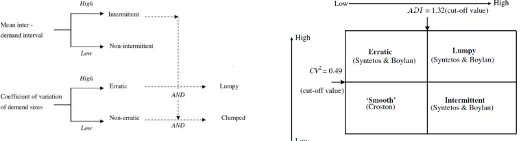
Syntetos et al. (2005) continued their work and compared three forecasting methods (SES, Croston’s method, and SBA) based on their theoretical MSE to identify the regions of their lesser MSE. They took into account two parameters to produce their classification scheme (the left side of Figure 1), namely the demand interval (ADI) and demand size variability (CV2). ADI measured the average number of time periods between two consecutive demands and CV represented the standard deviation of demand sizes divided by the average demand sizes when they occur.

(13)

3 and intermittent (but not very erratic). They concluded that SBA was theoretically expected to perform better than SES and Croston’s method when ADI>1.32 and/or CV2>0.49. For ADI≤1.32 and CV2≤0.49, Croston’s method was supposed to perform better than the other two methods. This condition was prevailed when all points in time were considered. Boylan et. al (2008) later demonstrated by empirical study that the approximate ADI range 1.18-1.86 is insensitive to issue points forecast accuracy.

Figure 1 Syntetos et. al demand categorization scheme (Boylan et. al (2008))

Croston’s Method and Syntetos-Boylan Approximation

Croston (1972) observed the inadequacy of SES to forecast items with intermittent demand, which resulted in excessive stock levels. To handle this problem, he suggested separate estimates of demand size and frequency. Furthermore, he modified the basic stock replenishment rules to incorporate his estimator.

In modeling process, Croston assumed that both demand sizes and intervals have constant means and variances (stationary) and are mutually independent. Demand was assumed to occur as a Bernoulli process, thus inter-demand intervals were assumed to be geometrically distributed. Furthermore, the demand sizes were assumed to follow the normal distribution (Boylan and Syntetos 2008).

Croston’s method works as follows. When demand occurs, SES estimates of the average demand size and the average inter-demand interval are updated. Otherwise, the estimates are the same as the previous ones. If demand occurs in every period, Croston’s forecasts are identical to those of SES (Boylan and Syntetos 2008).

In spite of its theoretical superiority, empirical evidence revealed modest improvements of Croston’s method over simpler forecasting techniques. Syntetos and Boylan (2001) tried to identify the cause of this discrepancy and found a mistake on mathematical derivation of Croston’s formulas. They then proposed a bias-adjusted estimator and compared the performance of the two estimators through simulation. The outcomes encouraged revision of Croston’s original estimate to overcome its inherent positive bias.

Mean Absolute Scaled Error (MASE)

(14)

4

independent of the scale of the data and is finite except when all historical data are equal. It is less than one if it is generated by a more accurate forecast than the average one-step naive forecast computed in-sample and vice versa. The MASE is simply the average of the absolute scaled error.

Mean Absolute Deviation to Mean Ratio (MAD-to-Mean)

Hoover (2006) recommended the use of MAD-to-Mean as an appropriate measure to asses forecast accuracy because it is scale independent and intuitively understandable to both managers and forecasters. This measure is always finite unless all historical data happen to be zero. Hyndman (2006) argued that MAD-to-Mean assumes the mean is stable over time, which is often the case with intermittent data.

Percentage Best (PBt)

Percentage best is defined as the percentage of times that one method performs better than all other methods. This non-parametric measure requires one or more descriptive accuracy measures, such as the MASE and MAD-to-Mean, to provide comparisons on the relative performance of every method in each one of the series. However, this measure gives no indication on how much one method outperforms the other methods (Syntetos and Boylan 2005).

METHODOLOGY

Data Sources

The data exercised in this study was queried from a branch office of a heavy equipment company in Indonesia. They were in forms of sales transaction record from January 2010 to June 2013. At first, they were pivoted for each parts number to obtain monthly order quantity (demand). All SKUs that were ordered at least once during 2012 were further considered. They consisted of bolt, cartridge, filter, piston, ring, valve, etc.

(15)

5 Methods

The procedures involved in this study are: 1. Demand Categorization

2 where N denote the number of periods with non-zero

demands, t and X refer to time period and demand size when they occur. Subsequently, each SKU is categorized based on the cut-off values suggested by Syntetos et al. (2005).

2. Demand Forecasting

Apply the four forecasting methods described in Table 1 to every demand series. The formulas of those methods are given in Table 2.

Table 1 Forecasting methods

Forecasting Methods Smoothing Constants (α)

Simple Moving Average 12-months span

Single Exponential Smoothing 0.05, 0.10, 0.15, 0.20

Croston’s Method 0.05, 0.10, 0.15, 0.20

Syntetos-Boylan Approximation 0.05, 0.10, 0.15, 0.20

Table 2 Formulas of forecasting methods

Forecasting Tt represent inter-demand interval between the latest and previous demand and forecasted inter-demand interval in period t. At last, dt symbolizes forecast of the demand rate in period t.

(16)

6

interval over the first 24 months are taken to be the initial SES estimates of demand size and inter-demand interval.

3. Forecasts Evaluation

Calculate the forecast errors (MASE, MAD-to-Mean, and PBt) of all demand series and asses the performance of the four forecasting methods. The descriptive measures, MASE and MAD-to Mean, are aggregated across series and the method that generates the lowest median is considered as the best. To determine the PBt across series, the minimum MASE and MAD-to-Mean of every forecasting method on each demand series are first calculated and then ranked. When ties occur on a series, all methods with minimum MASE or MAD-to-Mean value are tallied. The method that produces the highest PBt is regarded as the best method.

Finally, the best forecasting method on each category is compared with SMA. Two-sided Wilcoxon signed rank tests are conducted to test the median of pair-wise MAD-to-Mean difference between the best forecasting method and SMA across series. The null hypothesis is the median of differences between the two corresponding methods is equal to zero.

The test statistic (W) is obtained the following way. Initially, the signed differences on each series are calculated and their absolute values are ranked from smallest to largest across series. Afterward, the sign of the differences is assigned to the resulting rank associated with them and the sum of the ranks with positive and negative signs is computed. The smaller of the two sums is the test statistic. For large number of series (n), W∗ = W−n(n+1)/4

n n+1 (2n+1)/24 approximately follow standard normal distribution (Daniel 1990).

RESULTS AND DISCUSSIONS

Demand Categorization Results

A total of 9,308 SKUs have been forecasted, 7,432 of them fall into the intermittent category. The other 1,320 items are categorized as lumpy demand, while the remaining 279 and 277 items fall into the erratic and smooth category. Overall, the ADI ranges from 1 to 35 months with median 8.75 months and the CV2 ranges from 0 to 6.8 with median 0.12. The average demand per unit time ranges from 0.03 to 21,380.33 units per month.

(17)

7 Table 3 Properties of each demand category

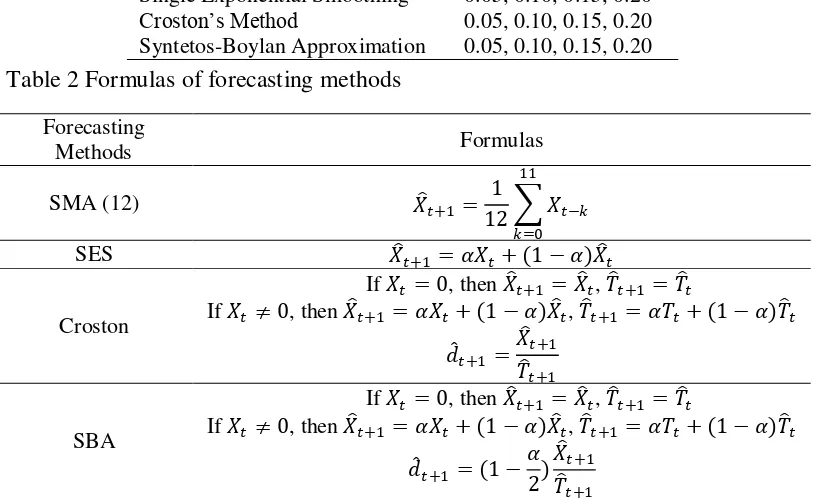
Demand Categories erratic and smooth category they pick SBA (α=0.20) as the best method, while for the lumpy category SMA is considered as the best. Slight disagreement is observed on intermittent category. The MASE of SBA (α=0.05) is the lowest across series, while SES (α=0.05) results in the lowest MAD-to-Mean followed by SBA (α=0.05).

On erratic category (Figure 2), SMA is better than smoothing methods for lower smoothing constants (α=0.05, 0.10) but worse for higher ones (α=0.10, 0.15). It can be seen from Figure 2 that SBA continually performs better than the rest smoothing methods, with one exception for its MASE at α=0.05 where SES is better. On lumpy category where SMA is the best, SES constantly performs as the second best followed by SBA and Croston as shown in Figure 3.

Figure 2 The median of MASE and MAD-to-Mean across erratic category series

(18)

8

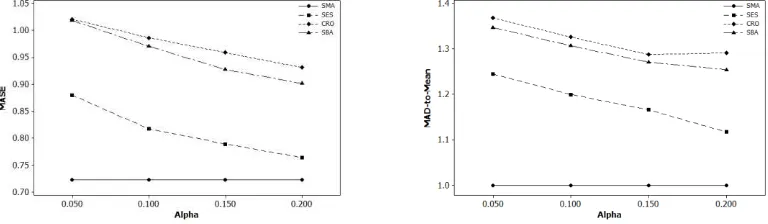
SBA once again performs better than the remaining forecasting methods on smooth category apart from its MASE at α=0.05 (Figure 4). This is also the case with intermittent category excluding its MAD-to-Mean at α=0.05 (Figure 5). It should be noticed from Figure 5 below that SES performance on intermittent category deteriorates greatly for alphas higher than 0.05.

Figure 4 The median of MASE and MAD-to-Mean across smooth category series

Figure 5 The median of MASE and MAD-to-Mean across intermittent category series

Higher smoothing constant is preferred for erratic, lumpy, and smooth category, where α=0.20 generally produces the best result. In contrast, lower smoothing constant (α=0.05) is found to be optimal for intermittent category. This study also finds that, for the same alpha values, SBA performs better than Croston in all cases. These outcomes can be verified from the line plots shown above.

On the whole, the MAD-to-Mean of lumpy category is the highest among other demand categories which makes this category hardest to forecast. As expected, the MAD-to-Mean of smooth category is found to be the lowest. Regarding the MASE results, intermittent category produces MASE across series which is considerably below the other three demand categories. This means that on this category the performance of all corresponding methods is the finest when compared to the naive forecasts.

Talking about the variation of MASE and MAD-to-Mean across series, the inter-quartile range (IQR) of MASE and MAD-to-Mean on lumpy and intermittent category is much higher than those of erratic and smooth category. This can be interpreted as SKUs on these categories are forecasted with various levels of accuracy. Perhaps this is contributed by the large number of items which fall in these categories.

(19)

9 method. Since SMA is the best on lumpy category, it is going to be compared with the second best method (SES with α=0.20). Exception is made on intermittent category, where SES (α=0.20) generates the lowest MAD-to-Mean. In its place, SBA (α=0.20) is going to be matched with SMA because of its more stable forecast errors across alpha values.

The two-sided Wilcoxon signed rank test results are reported in Table 4. All methods with exemption on lumpy category show significant improvement over SMA at 1% significance level. In addition, there is not enough evidence that SMA is better than SES (α=0.20) on lumpy category. Nevertheless, SMA is the one recommended here owing to its simple calculation.

Table 4 The Wilcoxon signed rank test results of each demand category

Demand Categories Wilcoxon Signed Ranked Tests ∗ Statistic P-value

Erratic SBA (α=0.20) vs. SMA 4.702 0.000

Lumpy SES (α=0.20) vs. SMA 0.338 0.735

Smooth SBA (α=0.20) vs. SMA 3.748 0.000

Intermittent SBA (α=0.05) vs. SMA 32.337 0.000

Percentage Best Results

The Percentage Best results based on MASE and MAD-to-Mean are alike, so they are averaged and rounded to the nearest half percentages in Table 5. This is in line with Syntetos and Boylan (2005) finding that PBt seems to be insensitive to the descriptive measure chosen. Additionally, the accuracy differences on MASE and MAD-to-Mean across series are not necessarily reflected on PBt, which only counts the number of series for which one method performs better than all other methods based on their MASE or MAD-to-Mean values.

Table 5 The PBt results of each demand category

Forecasting Methods Demand Categories

Erratic Lumpy Smooth Intermittent

SMA 18.0% 24.5% 16.0% 13.5%

SES 25.5% 31.0% 24.5% 34.5%

CRO 19.0% 16.5% 21.0% 8.0%

SBA 37.5% 28.0% 38.5% 44.0%

(20)

10

The forecast errors of all methods are still considerably high, which is probably attributable to the long forecast horizon. The benefits obtained from the above-discussed methods seem lost when forecasting is done for more than one period ahead. This is related to the ability of those methods which can only produce flat forecasts no matter how long the forecast horizon is. The best forecasting method for each demand category based on three error measures is recapped in Table 6.

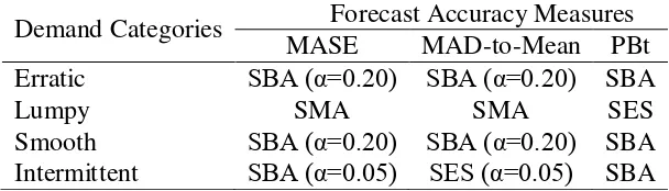
Table 6 The best forecasting method of each demand category

Demand Categories Forecast Accuracy Measures MASE MAD-to-Mean PBt Erratic SBA (α=0.20) SBA (α=0.20) SBA

Lumpy SMA SMA SES

Smooth SBA (α=0.20) SBA (α=0.20) SBA Intermittent SBA (α=0.05) SES (α=0.05) SBA

Based on this table, SBA (α=0.20) is recommended for both erratic and smooth category. Meanwhile, SBA (α=0.05) is advised for intermittent category considering SES deteriorating performance on higher alpha values. As for lumpy category, the hardest category to forecast, SMA is preferred than SES (α=0.20) on account of its simplicity. This is of course a rather surprising finding, which calls for more investigation. It should be pointed out that these outcomes may only be applicable to the current data set.

CONCLUSIONS AND EXTENSIONS

Conclusions

(21)

11 Extensions

Several extensions can be made for future studies. The optimization of the smoothing constants used to update forecasts has not been taken into consideration. Also, the effect of forecast lead time on forecast accuracy necessitates further assessment. More importantly, the forecasting implication of employing the recommended method on the company inventory system needs to be evaluated. To practitioners, what matters the most are stock control performance metrics such as inventory turnover and customer service level.

REFERENCES

Boylan JE, Syntetos AA. 2008. Forecasting for Inventory Management of Service Parts. In: Kobbacy KAH, Murthy DNP, editors. Complex System Maintenance Handbook. London (GB): Springer-Verlag. pp 479-508.

Boylan JE, Syntetos AA, Karakostas GC. 2008. Classification for Forecasting and Stock Control: A Case Study. J Opl Res Soc. 59: 473-481.

Croston JD. 1972. Forecasting and Stock Control for Intermittent Demands. Opl Res Q. 23: 289-304.

Daniel WW. 1990. Applied Nonparametric Statistics 2nd ed. Boston (US): PWS-Kent.

Hoover J. 2009. How to Track Forecast Accuracy to Guide Forecast Process Improvement. Foresight: the Int J Appl Forecast. 14: 17-23.

Hyndman RJ. 2006. Another Look at Forecast Accuracy Metrics for Intermittent Demand. Foresight: the Int J Appl Forecast. 4: 43-46.

Johnston FR, Boylan JE. 1996. Forecasting for Items with Intermittent Demand. J Opl Res Soc. 47: 113-121.

Syntetos AA, Boylan JE. 2001. On the Bias of Intermittent Demand Estimates. Int J Prod Econ. 71: 457-466.

Syntetos AA, Boylan JE. 2005. The Accuracy of Intermittent Demand Estimates. Int J Forecast. 21: 303-314.

(22)

12

Appendix 1 The MASE and MAD-to-Mean results of erratic category Forecasting Methods MASE MAD-to-Mean Median IQR Median IQR

SMA 0.795 0.531 0.640 0.364

SES (α=0.05) 0.882 0.688 0.688 0.517 SES (α=0.10) 0.826 0.551 0.640 0.425 SES (α=0.15) 0.778 0.539 0.615 0.385 SES (α=0.20) 0.765 0.559 0.607 0.381 CRO (α=0.05) 0.908 0.701 0.699 0.541 CRO (α=0.10) 0.840 0.600 0.650 0.487 CRO (α=0.15) 0.805 0.553 0.638 0.414 CRO (α=0.20) 0.778 0.566 0.618 0.406 SBA (α=0.05) 0.892 0.722 0.678 0.529 SBA (α=0.10) 0.815 0.547 0.635 0.475 SBA (α=0.15) 0.757 0.569 0.613 0.419 SBA (α=0.20) 0.736 0.572 0.585 0.427

Appendix 2 The PBt results of erratic category

Forecasting Methods PBt

MASE MAD-to-Mean

SMA 17.80% 17.97%

SES 25.64% 25.37%

CRO 19.28% 19.24%

(23)

13 Appendix 3 The MASE and MAD-to-Mean results of lumpy category

Forecasting Methods MASE MAD-to-Mean Median IQR Median IQR

SMA 0.723 0.722 1.000 0.636

SES (α=0.05) 0.880 1.071 1.245 1.650 SES (α=0.10) 0.817 0.866 1.200 1.259 SES (α=0.15) 0.789 0.789 1.166 0.984 SES (α=0.20) 0.764 0.779 1.117 1.000 CRO (α=0.05) 1.021 1.519 1.368 2.204 CRO (α=0.10) 0.987 1.372 1.326 2.078 CRO (α=0.15) 0.959 1.286 1.288 1.960 CRO (α=0.20) 0.931 1.235 1.292 1.884 SBA (α=0.05) 1.019 1.490 1.347 2.145 SBA (α=0.10) 0.971 1.311 1.307 2.057 SBA (α=0.15) 0.927 1.271 1.271 1.912 SBA (α=0.20) 0.902 1.184 1.254 1.828

Appendix 4 The PBt results of lumpy category

MASE MAD-to-Mean

SMA 24.47% 24.51%

SES 30.94% 30.92%

CRO 16.40% 16.56%

(24)

14

Appendix 5 The MASE and MAD-to-Mean results of smooth category Forecasting Methods MASE MAD-to-Mean

Median IQR Median IQR

SMA 0.863 0.570 0.504 0.337

SES (α=0.05) 0.911 0.603 0.499 0.386 SES (α=0.10) 0.863 0.553 0.500 0.348 SES (α=0.15) 0.863 0.543 0.500 0.324 SES (α=0.20) 0.882 0.533 0.487 0.331 CRO (α=0.05) 0.911 0.630 0.498 0.395 CRO (α=0.10) 0.891 0.548 0.492 0.344 CRO (α=0.15) 0.878 0.521 0.502 0.352 CRO (α=0.20) 0.890 0.528 0.511 0.349 SBA (α=0.05) 0.894 0.612 0.490 0.393 SBA (α=0.10) 0.863 0.535 0.486 0.346 SBA (α=0.15) 0.838 0.524 0.478 0.330 SBA (α=0.20) 0.818 0.546 0.464 0.341

Appendix 6 The PBt results of smooth category

MASE MAD-to-Mean

SMA 16.14% 16.31%

SES 24.41% 24.36%

CRO 21.06% 21.02%

(25)

15 Appendix 7 The MASE and MAD-to-Mean results of intermittent category

Forecasting Methods MASE MAD-to-Mean Median IQR Median IQR

SMA 0.688 0.733 1.000 0.667

SES (α=0.05) 0.550 0.866 0.831 1.271 SES (α=0.10) 0.620 0.756 1.037 1.017 SES (α=0.15) 0.688 0.884 1.161 1.047 SES (α=0.20) 0.707 0.938 1.229 1.465 CRO (α=0.05) 0.541 1.001 0.892 1.618 CRO (α=0.10) 0.552 0.986 0.921 1.587 CRO (α=0.15) 0.563 0.975 0.948 1.532 CRO (α=0.20) 0.591 0.964 0.979 1.495 SBA (α=0.05) 0.533 0.994 0.887 1.593 SBA (α=0.10) 0.543 0.982 0.899 1.540 SBA (α=0.15) 0.550 0.971 0.915 1.480 SBA (α=0.20) 0.555 0.951 0.925 1.473

Appendix 8 The PBt results of intermittent category Forecasting Methods PBt

MASE MAD-to-Mean

SMA 13.58% 13.63%

SES 34.61% 34.56%

CRO 8.03% 8.09%

(26)

16

BIOGRAPHY

Ryan Pasca Aulia was born in Padang as the eldest son of Ahmad Fauzan and Yasmurti Pertamasari on September 16 1993. He completed high school education from SMAN 10 Padang and MTsN Model Padang before pursuing his Bachelor of Statistics degree at Bogor Agricultural University in 2010. During his sophomore and junior years, he took some basic courses in Financial and Actuarial Mathematics.