arXiv:0903.4331v2 [stat.AP] 27 Jul 2009
Technical Report # KU-EC-09-4:
A Comparison of Analysis of Covariate-Adjusted Residuals and
Analysis of Covariance
E. Ceyhan
1∗, Carla L. Goad
2July 27, 2009
1Department of Mathematics, Ko¸c University, 34450, Sarıyer, Istanbul, Turkey.
2Department of Statistics, Oklahoma State University, Stillwater, OK 74078-1056, USA.
*corresponding author:
Elvan Ceyhan,
Dept. of Mathematics, Ko¸c University, Rumelifeneri Yolu, 34450 Sarıyer, Istanbul, Turkey
e-mail: [email protected]
phone: +90 (212) 338-1845
fax: +90 (212) 338-1559
short title: ANOVA on Covariate-Adjusted Residuals and ANCOVA
Abstract
Various methods to control the influence of a covariate on a response variable are compared. In particular, ANOVA with or without homogeneity of variances (HOV) of errors and Kruskal-Wallis (K-W) tests on covariate-adjusted residuals and analysis of covariance (ANCOVA) are compared. Covariate-adjusted residuals are obtained from the overall regression line fit to the entire data set ignoring the treatment levels or factors. The underlying assumptions for ANCOVA and methods on covariate-adjusted residuals are determined and the methods are compared only when both methods are appropriate. It is demonstrated that the methods on covariate-adjusted residuals are only appropriate in removing the covariate influence when the treatment-specific lines are parallel and treatment-specific covariate means are equal. Empirical size and power performance of the methods are compared by extensive Monte Carlo simulations. We manipulated the conditions such as assumptions of normality and HOV, sample size, and clustering of the covariates. The parametric methods (i.e., ANOVA with or without HOV on covariate-adjusted residuals and ANCOVA) exhibited similar size and power when error terms have symmetric distributions with variances having the same functional form for each treatment, and covariates have uniform distributions within the same interval for each treatment. For large samples, it is shown that the parametric methods will give similar results if sample covariate means for all treatments are similar. In such cases, parametric tests have higher power compared to the nonparametric K-W test on covariate-adjusted residuals. When error terms have asymmetric distributions or have variances that are heterogeneous with different functional forms for each treatment, ANCOVA and analysis of covariate-adjusted residuals are liberal with K-W test having higher power than the parametric tests. The methods on covariate-adjusted residuals are severely affected by the clustering of the covariates relative to the treatment factors, when covariate means are very different for treatments. For data clusters, ANCOVA method exhibits the appropriate level. However such a clustering might suggest dependence between the covariates and the treatment factors, so makes ANCOVA less reliable as well. Guidelines on which method to use for various cases are also provided.
1
Introduction
In an experiment, the response variable may depend on the treatment factors and quite often on some external factor that has a strong influence on the response variable. If such external factors are qualitative or discrete, thenblocking can be performed to remove their influence. However, if the external factors are quantitative
and continuous, the effect of the external factor can be accounted for by adopting it as acovariate (Kuehl
(2000)), which is also called aconcomitant variable(Ott (1993), Milliken and Johnson (2002)). Throughout
this article, a covariate is defined to be a variable that may affect the relationship between the response variable and factors (or treatments) of interest, but is not of primary interest itself. Maxwell et al. (1984) compared methods of incorporating a covariate into an experimental design and showed that it is not correct to consider the correlation between the dependent variable and covariate in choosing the best technique. Instead, they recommend considering whether scores on the covariate are available for all subjects prior to assigning any subject to treatment conditions and whether the relationship of the dependent variable and covariate is linear.
In various disciplines such as ecology, biology, medicine, etc. the goal is comparison of a response variable among several treatments after the influence of the covariate is removed. Different techniques are used or suggested in statistical and biological literature to remove the influence of the covariate(s) on the response variable (Huitema (1980)). For example in ecology, one might want to compare richness-area relationships among regions, shoot ratios of plants among several treatments, and of C:N ratios among sites (Garcia-Berthou (2001)). There are three main statistical techniques for attaining that goal: (i) analysis of the ratio of response to the covariate; (ii) analysis of the residuals from the regression of the response with the covariate; and (iii) analysis of covariance (ANCOVA).
Analysis of the ratios is perhaps the oldest method used to remove the covariate effect (e.g., size effect in biology) (see Albrecht et al. (1993) for a comprehensive review). Although many authors recommend its disuse (Packard and Boardman (1988), Atchley et al. (1976)), it might still appear in literature on oc-casion (Albrecht et al. (1993)). For instance, in physiological and nutrition research, the data are scaled by taking the ratio of the response variable to the covariate. Using the ratios in removing the influence of the covariate on the response depends on the relationship between the response and the covariate vari-ables (Raubenheimer and Simpson (1992)). Regression analysis of a response variable on the covariate(s) is
common to detect such relationships, which are categorized as isometric or allometric relationships (Small
(1996)). Isometryoccurs when the relationship between a response variable and the covariate is linear with
a zero intercept. If the relationship is nonlinear or if there is a non-zero intercept, it is called allometry. In
allometry, the influence of the covariate cannot be removed by taking the ratio of the response to the
covari-ate. In both of allometry and isometry cases, ANOVA on ratios (i.e., response/covariate values) introduces
heterogeneity of variances in the error terms which violates an assumption of ANOVA (with homogeneity of variances (HOV)). Hence, ANOVA on ratios may give spurious and invalid results for treatment comparisons, so ANCOVA is recommended over the use of ratios (Raubenheimer and Simpson (1992)). See Ceyhan (2000) for a detailed discussion on the use of ratios to remove the covariate influence.
An alternative method to remove the effect of a covariate on the response variable in biological and ecological research is the use of residuals (Garcia-Berthou (2001)). In this method an overall regression line is fitted to the entire data set and residuals are obtained from this line (Beaupre and Duvall (1998)).
These residuals will be referred to ascovariate-adjusted residuals, henceforth. This method was recommended
in ecological literature by Jakob et al. (1996) who called it “residual index” method. Then treatments are compared with ANOVA with HOV on these residuals.
assumptions even if the original data did satisfy them. In fact, Maxwell et al. (1985) also demonstrated the inappropriateness of ANOVA on residuals.
Although ANCOVA is a well-established and highly recommended tool, it also has critics. However, the main problem in literature is not the inappropriateness of ANCOVA, rather its misuse and misinterpretation. For example, Rheinheimer and Penfield (2001) investigated how the empirical size and power performances of ANCOVA are affected when the assumptions of normality and HOV, sample size, number of treatment groups, and strength of the covariate-dependent variable relationship are manipulated. They demonstrated
that for balanced designs, the ANCOVA F test was robust and was often the most powerful test through
all sample-size designs and distributional configurations. Otherwise it was not the best performer. In fact, the assumptions for ANCOVA are crucial for its use; especially, the independence between the covariate and the treatment factors is an often ignored assumption resulting incorrect inferences (Miller and Chapman (2001)). This violation is very common in fields such as psychology and psychiatry, due to nonrandom group assignment in observational studies, and Miller and Chapman (2001) also suggest some alternatives for such cases. Hence the recommendations in favor on ANCOVA (including ours) are valid only when the underlying assumptions are met.
In this article, we demonstrate that it is not always wrong to use the residuals. We also discuss the differences between ANCOVA and analysis of residuals, provide when and under what conditions the two procedures are appropriate and comparable. Then under such conditions, we not only consider ANOVA (with HOV), but also ANOVA without HOV and Kruskal-Wallis (K-W) test on the covariate-adjusted residuals. We provide the empirical size performance of each method under the null case and the empirical power under various alternatives using extensive Monte Carlo simulations.
The nonparametric analysis by K-W test on the covariate-adjusted residuals is actually not entirely non-parametric, in the sense that, the residuals are obtained from a fully parametric model. However, when the covariate is not continuous but categorical data with ordinal levels, then a nonparametric version of ANCOVA can be performed (see, e.g., Akritas et al. (2000) and Tsangari and Akritas (2004a)). Further, the nonpara-metric ANCOVA model of Akritas et al. (2000) is extended to longitudinal data for up to three covariates (Tsangari and Akritas (2004b)). Additionally, there are nonparametric methods such as Quade’s procedure, Puri and Sen’s solution, Burnett and Barr’s rank difference scores, Conover and Iman’s rank transformation test, Hettmansperger’s procedure, and the Puri-Sen-Harwell-Serlin test which can be used as alternatives to ANCOVA (see Rheinheimer and Penfield (2001) for the comparison of the these tests with ANCOVA and relevant references). In fact, Rheinheimer and Penfield (2001) showed that with unbalanced designs, with variance heterogeneity, and when the largest treatment-group variance was matched with the largest group sample size, these nonparametric alternatives generally outperformed the ANCOVA test.
The methods to remove covariate influence on the response are presented in Section 2, where the ANCOVA method, ANOVA with HOV and without HOV on covariate adjusted residuals, and K-W test on covariate-adjusted residuals are described. A detailed comparison of the methods, in terms of the null hypotheses, and conditions under which they are equivalent are provided in Section 3. The Monte Carlo simulation analysis used for the comparison of the methods in terms of empirical size and power is provided in Section 4. A discussion together with a detailed guideline on the use of the discussed methods is provided in Section 5.
2
ANCOVA and Methods on Covariate-Adjusted Residuals
In this section, the models and the corresponding assumptions for ANCOVA and the methods on covariate-adjusted residuals are provided.
2.1
ANCOVA Method
For convenience, only ANCOVA with a one-way treatment structure in a completely randomized design and a single covariate is investigated. A simple linear relationship between the covariate and the response for each treatment level is assumed.
replicates for each covariate value for treatment levelifor i= 1,2, . . . , tandj = 1,2, . . . , ni where ni is the
number of distinct covariate values at treatment level i. Letn be the total number of observations in the
entire data set then si =Pnj=1i rij andn =Pti=1si. ANCOVA fits a straight line to each treatment level.
These lines can be modeled as
Yijk = µi+βiXij+eijk (1)
where Xij is the jth value of the covariate for treatment level i, Yijk is the kth response at Xij, µi is the
intercept and βi is the slope for treatment level i, and eijk is the random error term for i = 1,2, . . . , t,
j = 1,2, . . . , ni, and k = 1,2, . . . , rij. The assumptions for the ANCOVA model in Equation (1) are: (a)
The Xij (covariate) values are assumed to be fixed as in regression analysis (i.e., Xij is not a random
variable). (b) eijk
iid
∼N 0, σ2e
for all treatments whereiid∼ stands for “independently identically distributed
as”. This implies Yijk are independent of each other and Yijk ∼N µi+βiXij, σ2e
. (c) The covariate and the treatment factors are independent. Then the straight line fitted by ANCOVA to each treatment can be
written asYbij = µbi+βbiXij, whereYbij is the predicted response for treatmentiatXij,µbi is the estimated
intercept, andβbi is the estimated slope for treatmenti.
In the analysis, these fitted lines can then be used to test the following null hypotheses:
(i)Ho:β1=β2=· · ·=βt= 0 (All slopes are equal to zero).
If Ho is not rejected, then the covariate is not necessary in the model. Then a regular one-way ANOVA can
be performed to test the equality of treatment means.
(ii)Ho:β1=β2=· · ·=βt(The slopes are equal).
Depending on the conclusion reached here, two types of models are possible for linear ANCOVA models
-parallel lines and non-parallel lines models. If Ho in (ii) is not rejected, then the lines are parallel, otherwise
they are nonparallel (Milliken and Johnson (2002)). Throughout the article the terms “parallel lines models (case)” and “equal slope models (case)” will be used interchangeably. The same holds for “nonparallel lines models (case)” and “unequal slopes models (case)”.
The parallel lines model is given by
Yijk = µi+β Xij+eijk, (2)
where βis the common slope for all treatment levels. With this model, testing the equality of the intercepts,
Ho:µ1=µ2=· · ·=µt, is equivalent to testing the equality of treatment means at any value of the covariate.
For the nonparallel lines case, the model is as in Equation (1) with at least oneβi being different for some
i= 1,2, . . . , t. So the comparison of treatments may give different results at different values of the covariate.
2.2
Analysis of Covariate-Adjusted Residuals
First an overall regression line is fitted to the entire data set as:
b
Yij=µb+βb∗Xij, fori= 1,2, . . . , tandj= 1,2, . . . , ni, (3)
where µb is the estimated overall intercept and βb∗ is the estimated overall slope. The residuals from this
regression line are calledcovariate-adjusted residuals and are calculated as:
Rijk=Yijk−Ybij=Yijk−µb−βb∗Xij,fori= 1,2, . . . , t,j= 1,2, . . . , ni, andk= 1,2, . . . , rij, (4)
whereRijk is thekthresidual of treatment level iatXij.
2.2.1 ANOVA with or without HOV on Covariate-Adjusted Residuals
The means model and assumptions for the one-way ANOVA with HOV on these covariate-adjusted resid-uals are:
Rijk = ρi+εijk, fori= 1,2, . . . , t,j= 1,2, . . . , ni,andk= 1,2, . . . , rij, (5)
where ρi is the mean residual for treatment i, εijk are the (independent) random errors such that εijk ∼
N 0, σ2
ε
. Notice the common variance σ2
ε for all treatment levels. However, Rijk are not independent of
each other, sincePti=1Pni
j=1
Prij
k=1Rijk= 0, which also implies that the overall mean of the residuals is zero.
Hence the model in Equation (3) and an effects model for residuals are identically parameterized.
For the nonparallel lines model in Equation (1), the residuals in Equation (4) will take the form:
Rijk=Yijk−Ybij =µi+βiXij+eijk−
b
µ+βb∗X
ij
= (µi−µb) +
βi−βb∗
Xij+eijk.
Hence, the influence of the covariate will be removed if and only if
b
β∗= β
i for all i= 1,2, . . . , t. (6)
Then taking covariate-adjusted residuals can only remove the influence of the covariate when the treatment-specific lines in Equation (1) and the overall regression in Equation (3) are parallel. Notice that the residuals from the treatment-specific models in Equation (1) cannot be used as response values in an ANOVA with HOV, because treatment sums of squares of such residuals are zero (Ceyhan (2000)).
In ANOVA without HOV on covariate-adjusted residuals, the only difference from ANOVA with HOV
is that εijk are the (independent) random errors such thatεijk ∼ N 0, σi2
. Notice the treatment-specific
variance termσi2; i.e., the homogeneity of the variances is not necessarily assumed in this model.
Kruskal-Wallis (K-W) test is an extension of the Mann-Whitney U test to three or more groups; and
for two groups K-W test and Mann-Whitney U test are equivalent (Siegel and Castellan Jr. (1988)). K-W
test on the covariate-adjusted residuals which are obtained as in model (4) tests the equality of the residual distributions for all treatment levels. Notice that contrary to the parametric models and tests in previous sections, only the distributional equality is assumed, neither normality nor HOV.
3
Comparison of the Methods
ANOVA with or without HOV or K-W test on covariate-adjusted residuals and ANCOVA can be compared when the treatment-specific lines and the overall regression line are parallel. The null hypotheses tested by “ANCOVA”, “ANOVA with or without HOV”, and “K-W test” on covariate-adjusted residuals are
Ho:µ1=µ2=· · ·=µt (Intercepts are equal for all treatments.) (7)
Ho:ρ1=ρ2=· · ·=ρt(Residual means are equal for all treatments.) (8)
and
Ho:FR1 =FR2 =· · ·=FRt (Residuals have the same distribution for all treatments.), (9)
respectively.
For more than two treatments the assumption of parallelism is less likely to hold, since only two lines with different slopes are sufficient to violate the condition. With two treatments, the null hypotheses tested by ANCOVA, ANOVA with or without HOV and K-W test on covariate-adjusted residuals will be
Ho:µ1=µ2 (orµ1−µ2= 0) (10)
Ho:ρ1=ρ2 (orρ1−ρ2= 0) (11) and
Ho:FR1 =FR2 (orR1
d
respectively, where= stands for “equal in distribution”.d
In Equation (11), ρi can be estimated by the sample residual mean, Ri... Combining the expressions in
(4) and (5), the residuals can be rewritten as
Rijk=ρi+εijk=Yijk−Ybij = (µi+βiXij+eijk)−
covariate-adjusted residuals, taking the expectations in (13) yields
ERi..
Using condition (6) and repeating the above argument for all pairs of treatments, the condition in (15) can be extended to more than two treatments.
Notice that the conditions that will imply (15) will also imply the equivalence of the hypotheses in (10) and (11). The overall regression slope can be estimated as
b
whereX.. is the overall covariate mean,Y...is the overall response mean, and
E∗
Furthermore the treatment-specific slope used in model (1) is estimated as
b
, and Yi.. is the mean response for treatment i. Substituting Yijk =
b
µi+βbiXij+R′ijk,i= 1,2,j= 1,2, . . . , ni, andk= 1,2, . . . , rij in Equation (16) whereµbi is the estimated
intercept for treatment leveli, andR′
ijk is the kth residual atXij in model (1), the estimated overall slope
becomes βb∗=
. With some rearrangements, we get
b
= 0, taking the expectations of both sides of (17) yields
UnderHo:µ1=µ2, (18) reduces toβ∗=βi iff
treatment-specific lines are parallel and treatment-specific means are equal which implies the condition stated in (6).
In general forttreatments, the hypotheses in (7) and (8) can be tested using anF test statistics. Ho in
(7) can be tested by
F = M ST rt
M SE , (20)
where M ST rt is the mean square treatment for response values, and M SE is the mean square error for
response values. These mean square terms can be calculated as:
M ST rt=
Similarly, Hoin (8) can be tested by
F∗= M ST rt∗
M SE∗ , (21)
where M ST rt∗ is the mean square treatment for covariate-adjusted residuals, and M SE∗ is the mean
square error for covariate-adjusted residuals. These mean square terms can be calculated as M ST rt∗ =
Pt
and Beaupre and Duvall (1998) used the method without such an adjustment. That is, in both sources
F(t−1, n−t) is used for inference. So, in this articledf forM SE∗has been set at (n−t) as in literature.
Notice that, theF-statistics in (20) and (21) become
and
F∗=
Pt i=1
Pni
j=1rij h
Yi..−Y...
−βb∗ X
i.−X.. i2
(t−1)
Pt i=1
Pni
j=1
Prij
k=1
h
Yijk−Yi..
−βb∗ Xij−Xi.i
2
(n− t)
, (23)
respectively. For two treatments, t = 2 will be used in Equations (22) and (23), then the test statistics will
be distributed asF ∼F(1, n−3) and F∗ ∼ F(1, n−2), and they can be used to test the hypotheses in
Equations (10) and (11), respectively. Furthermore, with two treatments, note thatF =d T2(n−3) and
F∗ =d T2(n−2) and T (n) is the t-distribution with n df. As n → ∞, both F and F∗ will converge in
distribution to χ21. So F and F∗ will have similar observed significance levels (i.e., p-values) and similar
scores for largen. Similar decisions for testing (10) and (11) will be reached if the calculated test statistics
are similar; i.e., F ≈F∗ for large n. Likewise,F in (20) andF∗ in (21) will have similar distributions for
largen.
For the case of two treatments, comparingF andF∗, it can be seen thatF andF∗ are similar ifβb∗≈βb
i
for largen. The same argument holds for the test statistics in the general case of more than two treatments
for largen. The test statistics will lead to similar decisions, if βb∗ ≈βb
i as n increases. That is, the overall
regression line fitted to the entire data set should be approximately parallel to the fitted treatment-specific
regression lines for the test statisticsF andF∗to be similar. Ifβb∗≈βb
i, then ANOVA with or without HOV
on covariate-adjusted residuals and ANCOVA will give similar results. Consequently, it is expected that the ANCOVA and ANOVA with HOV or without HOV methods give similar results as treatment-specific covariate means gets closer for the parallel lines case.
The above discussion is based on normality of error terms with HOV. Without HOV thedfof theF-tests
are calculated with Satterthwaite approximation (Kutner et al. (2004)). On the other hand, K-W test does
require neither normality nor HOV, but implies a more general hypothesisHo:FR1 =FR2, in the sense that
Ho would implyHo:ρ1=ρ2 without the normality assumption. However, the null hypothesis in Equation
(11) implicitly assumes normality.
4
Monte Carlo Simulation Analysis
Throughout the simulation only two treatments (t = 2) are used for the comparison of methods. In the
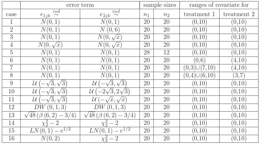
simulation, sixteen different cases are considered for comparison (see Table 1).
4.1
Sample Generation for Null and Alternative Models
Without loss of generality, the slope in model (2) is arbitrarily taken to be 2 and the intercept is chosen to be 1. So the response values for the treatments are generated as
(i)Y1jk= 1 + 2X1j+e1jk,j = 1,2, . . . , n1 andk= 1,2, . . . , r1j for treatment 1 (24)
withe1jk iid∼F1, whereF1is the error distribution for treatment 1.
(ii)Y2jk= (1 + 0.02q) + 2X2j+e2jk,j= 1,2, . . . , n2 andk= 1,2, . . . , r2j for treatment 2 (25)
withe2jk iid∼ F2, where F2 is the error distribution for treatment 2 andqis introduced to obtain separation
between the parallel lines. In (24) and (25),Xij is the jth generated value of the covariate in treatment i,
Yijk is the response value for treatment level i at Xij for i = 1,2, eijk is thekth random error term. The
covariate ranges, sample sizes (n1 and n2), error distributions (F1 and F2) for the two treatments, and the
number of replicates (reps) at each value ofXij are summarized in Table 1. In the context of model (2) the
common slope is β = 2, and µ1 = 1 and µ2 = (1 + 0.02q) are the intercepts for treatment levels 1 and 2,
respectively.
Then as qincreases the treatment-specific response means become farther apart at each covariate value
and efficiency of the simulation process. qis incremented from 1 to mu in case-u, for u= 1,2, ..., 16 (Table
1) where mu is estimated by the standard errors of the intercepts of the treatment-specific regression lines.
In the simulation no further values ofq are chosen when the power is expected to approach 1.00 that occurs
when the intercepts are approximately 2.5 standard errors apart, as determined by equating the intercept
difference, 0.02q= 2.5sµbi, withqreplaced bymu. A pilot sample of size 6000 is generated (q= 0,1,2,3,4,5
with 1000 samples at each q), and maximum of the standard errors of the intercepts is recorded. Then
mu∼= 2.5 maxi(sµbi)/0.02 fori= 1,2 in case u.
All cases labeled with “a” have one replicate and all cases labeled with “b” have two replicates per covariate
value, henceforth. For example, in case 1a the most general case is simulated withiid N(0,1) error variances,
and 20 uniformly randomly generated covariate values in the interval (0,10) for both treatments. In case 1b,
the data is generated as in case 1a with two replicates per covariate value.
In cases 1, 5-8, 9, and 12-16, error variances are homogeneous; in cases 1, and 5-8 error terms are generated as iid N(0,1). In case 9, error terms are generated as iid U −√3,√3; in case 12, error terms are iid
DW(0,1,3), double-Weibull distribution with location parameter 0, scale parameter 1, and shape parameter
3 whose pdf isf(x) = 3
2x
2exp
−|x|3 for all x; in case 13, error terms are iid√48 (β(6,2)−3/4) where
β(6,2) is the Beta distribution with shape parameters 6 and 2 whose pdf isf(x) = 42x5(1−x)I(0< x <1)
whereI(·) is the indicator function; in case 14, error terms areiidχ22−2 whereχ22is the chi-square distribution
with 2df; in case 15, error terms areiid LN(0,1)−e1/2 where LN(0,1) is the log-normal distribution with
location parameter 0 and scale parameter 1 whose pdf is f(x) = 1
x√2πexp
−12(logx)2
I(x >0), and in
case 16, error terms areiidN(0,2) for treatment 1 and iidχ22−2 for treatment 2.
In cases 2-4 heterogeneity of variances for normal error terms is introduced either by unequal but constant
variances (case 2), unequal but a combination of constant and x-dependent variances (case 3), or equal
and x-dependent variances (case 4). In case 10 error terms are iid U −√3,√3 for treatment 1 and iid
U −2√3,2√3for treatment 2; in case 11, error terms areiidU −√3,√3treatment 1 andiidU(−√x,√x)
for treatment 2.
The choice of constant variances is arbitrary, but the error term distributions for constant variance cases are
picked so that their variances are roughly between 1 and 6. However,x-dependence of variances is a realistic
but not a general case, since any function ofxcould have been used. For example, Beaupre and Duvall (1998)
who explored the differences in metabolism (O2consumption) of the Western diamondback rattlesnakes with
respect to their sex, the O2consumption was measured for males, non-reproductive females, and vitellogenic
females. To remove the influence of body mass which was deemed as a covariate on O2consumption, ANOVA
with HOV on covariate-adjusted residuals was performed. In their study, the variances of O2 consumption
for sexual groups have a positive correlation with body mass. In this study,√xis taken as the variance term
to simulate such a case. Heterogeneity of variances conditions violate one of the assumptions for ANCOVA and ANOVA with HOV on covariate-adjusted residuals, and are simulated in order to evaluate the sensitivity of the methods to such violations. The unequal variances in cases 2 and 3 were arbitrarily assigned to the treatments since all the other restrictions are the same for treatments at each of these cases. In case 5, different sample sizes are taken from that of other cases to see the influence of unequal sample sizes.
In cases 1-8, error terms are generated from a normal distribution. In cases 9-15, non-normal distributions for error generation are employed. In cases 9-12, the distribution of the error variances are symmetric around 0, while in cases 13-15 the distributions of the error terms are not symmetric around 0. Notice that cases 13-15 are normalized to have zero mean, and furthermore case 13 is scaled to have unit variance. The influence of non-normality and asymmetry of the distributions are investigated in these cases. In case 16, the influence of distributional differences (normal vs asymmetric non-normal) in the error term is investigated.
In cases 1-5 and 9-16, covariates are uniformly randomly generated, without loss of generality, in (0,10),
hence X1. ≈ X2. is expected to hold. In these cases the influence of replications (or magnitude of equal
randomly generated within (0,6) for treatment 1, and (4,10) for treatment 2, soX1.andX2.are expected to
be different. In fact, this case is expected to contain the largest difference betweenX1.andX2.. See Figure
1 for a realization of case 6. In case 7 treatment 1 has two clusters, such that each treatment 1 covariate
is randomly assigned to either (0,3) or (7,10) first, then the covariate is uniformly randomly generated in
that interval. Treatment 2 covariates are generated uniformly within the interval of (4,10). Note thatX1.
and X2. are expected to be very different, but not as much as case 6. See Figure 2 for a realization of
case 7. Notice that the second cluster of treatment 1 is completely inside the covariate range of treatment 2. These choices of clusters are inspired by the research of Beaupre and Duvall (1998) which dealt with O2 consumption of rattlesnakes. In case 8 treatment 1 has two clusters, each treatment 1 covariate is uniformly
randomly generated in the randomly selected interval of either (0,4) or (6,10). Treatment 2 covariates are
uniformly randomly generated in the interval (3,7). Hence X1. andX2. are expected to be similar. Notice
that treatment 2 cluster is in the middle of the treatment 1 clusters with mild overlaps.
4.2
Monte Carlo Simulation Results
In this section, the empirical size and power comparisons for the methods discussed are presented.
4.2.1 Empirical Size Comparisons
In the simulation process, to estimate the empirical sizes of the methods in question, for each case enumerated
in Table 1,Nmc= 10000 samples are generated with q= 0 using the relationships in (24) and (25). Out of
these 10000 samples the number of significant treatment differences detected by the methods is recorded. The number of differences detected concurrently by each pair of methods is also recorded. The nominal significance
level used in all these tests isα= 0.05. Based on these detected differences, empirical sizes are calculated as
b
αi=νi/Niwhereνiare number of significant treatment differences detected by methodiwith method 1 being
ANCOVA, method 2 being ANOVA with HOV, method 3 being to ANOVA without HOV, and method 4 being K-W test on covariate-adjusted residuals. Furthermore the proportion of differences detected concurrently by
each pair of methods isαbi,j=vi,j/Nmc, whereNmc= 10000 andνi,j is the number of significant treatment
differences detected by methodsi,j, with i6=j.For largeNmc,αbi∼˙N(αi, σ2αi),i= 1,2,3,4, where ˙∼stands
for “approximately distributed as”,αi is the proportion of treatment differences,σ2αi=αi(1−αi)/Nmcis the
variance of the unknown proportion,αiwhose estimate isαbi. Using the asymptotic normality of proportions
for largeNmc, the 95% confidence intervals are constructed for empirical sizes of the methods (not presented)
to see whether they contain the nominal significance level, 0.05 and the 95% confidence interval for the difference in the proportions (not presented either) to check whether the sizes are significantly different from each other.
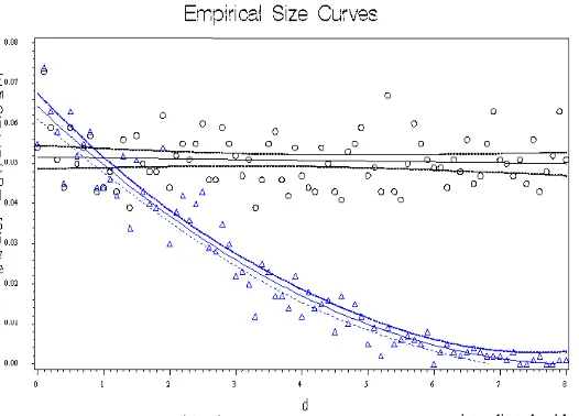
size for ANCOVA is stable about the desired nominal level 0.05. K-W test has the desired level when error terms have symmetric and identical distributions, is liberal when errors have the same distribution without HOV and different distributions, and is conservative when errors have asymmetric distributions provided the covariates have similar means. But when the covariate means are very different, KW test is also extremely conservative (see cases 6 and 7).
Moreover, observe that when the covariates have similar means, ANCOVA and ANOVA (with or without HOV) methods have similar empirical sizes. These three methods have similar sizes as K-W test when the error distributions have HOV. Without HOV, K-W test has significantly larger empirical size. When the covariate means are considerably different, ANCOVA method has significantly larger size than others. ANOVA with or without HOV methods have similar empirical sizes for all cases.
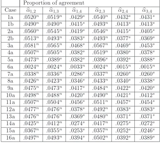
As seen in Table 3, the proportion of agreement between the empirical size estimates are usually not significantly different from the minimum of each pair of tests for ANCOVA and ANOVA with or without HOV, but the proportion of agreement is usually significantly smaller for the cases in which K-W test is compared with others. Therefore, when covariate means are similar, ANCOVA and ANOVA with or without HOV have the same null hypothesis, with similar acceptance/rejection regions, while K-W test has a different null hypothesis hence different acceptance/rejection regions. When covariate means are different, ANCOVA and ANOVA methods have different acceptance/rejection regions, and K-W test has a different null hypothesis. Both ANOVA methods have the same null hypothesis, and have similar acceptance/rejection regions for this simulation study.
4.2.2 Empirical Power Comparisons
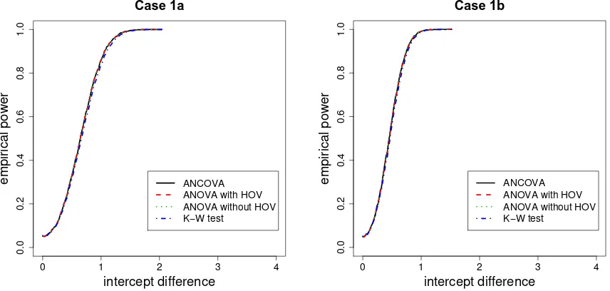
The empirical power curves are plotted in Figures 4, 5, 6, and 7. Empirical power corresponds toβbi,i= 1,2.
The value on the horizontal axis is defined to be intercept difference (i.e., 0.02q) as in (25). Then the empirical
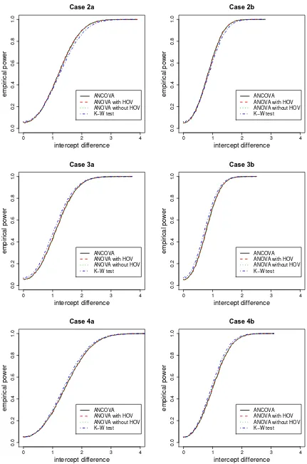
power curves are plotted against the simulated intercept difference values. In these figures the empirical power curve for a case labeled with “a” is steeper and approaches to 1.00 faster than that of the case labeled with “b” for the same case number, due to the fact that “b”-labeled cases have two replicates with the rest of the restrictions identical to the preceding “a”-labeled cases. Only cases labeled with “a” and “b” in case 1 are presented in Figure 4. For other cases, plot for only “a”-labeled case is presented.
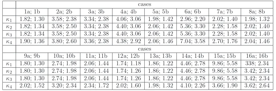
The first intercept difference value at which the power reaches 1 are denoted as κ and are provided in
5
Discussion and Conclusions
In this article, we discuss various methods to remove the covariate influence on a response variable when testing for differences between treatment levels. The methods considered are the usual ANCOVA method and the analysis of covariate-adjusted residuals using ANOVA with or without homogeneity of variances (HOV) and Kruskal-Wallis (K-W) test. The covariate-adjusted residuals are obtained from the fitted overall regression line to the entire data set (ignoring the treatment levels). For covariate-adjusted residuals to be appropriate for removing the covariate influence, the treatment-specific lines and the overall regression line should be parallel. On the other hand, ANCOVA can be used to test the equality of treatment means at specific values of the covariate. Furthermore, the use of ANCOVA is extended to the nonparallel treatment-specific lines also (Kowalski et al. (1994)).
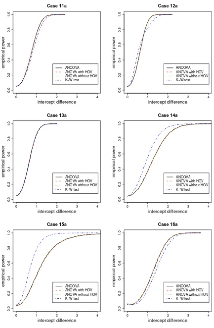
The Monte Carlo simulations indicate that when the covariates have similar means and have similar dis-tributions (with or without HOV), ANCOVA, ANOVA with or without HOV methods have similar empirical sizes; and K-W test is sensitive to distributional differences, since the null hypotheses for the first three tests are about same while it is more general for K-W test. When the treatment-specific lines are parallel, treatment-specific covariate ranges and covariate distributions are similar. ANCOVA and ANOVA with or without HOV on covariate-adjusted residuals give similar results if error variances have symmetric distribu-tions with or without HOV and sample sizes are similar for treatments; give similar results if error variances are homogeneous and sample sizes are different but large for treatments. In these situations, parametric tests are more powerful than K-W test. The methods give similar results but are liberal if error variances are heterogeneous with different functional forms for treatments. In these cases, usually K-W test has better performance.
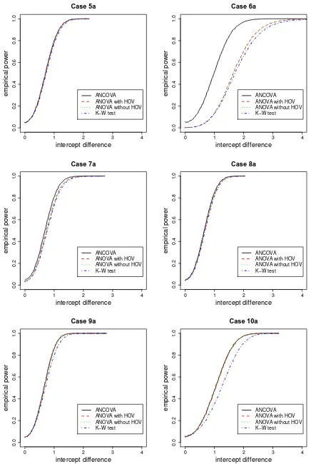
When the treatment-specific lines are parallel, but treatment-specific covariate ranges are different; i.e., there exist clustering of the covariate relative to the treatment factors, ANCOVA and ANOVA on covariate-adjusted residuals yield similar results if treatment-specific covariate means are similar, very different results if treatment-specific covariate means are different since overall regression line will not be parallel to the treatment-specific lines. In such a case, methods on covariate-adjusted residuals tend to be extremely
con-servative whereas the size of ANCOVAF test is about the desired nominal level. Moreover, ANCOVA is
much more powerful than ANOVA on covariate-adjusted residuals in these cases. The power of ANOVA on covariate-adjusted residuals gets closer to that of ANCOVA, as the difference between the treatment-specific covariate means gets smaller. However, in the case of clustering of covariates relative to the treatments, one should also exercise extra caution due to the extrapolation problem. Moreover in practice, such clustering is suggestive of an ignored grouping factor as in blocking. The discussed methods are meaningful only within the overlap of the clusters or in the close vicinity of them. However, when there are clusters for the groups in terms of the covariate, it is very likely that covariate and the group factors are dependent, which violates an assumption for ANCOVA. When this dependence is strong then ANCOVA method will not be appropriate. On the other hand, the residual analysis is extremely conservative which might be viewed as an advantage in order not to reach spurious and confounded conclusions in such a case.
The ANCOVA models can be used to estimate the treatment-specific response means at specific values of the covariate. But the ANOVA model on covariate-adjusted residuals should be used together with the fitted overall regression line in such an estimation, as long as condition (7) holds.
Different treatment-specific covariate distributions within the same interval or different intervals might also cause treatment-specific covariate means to be different. In such a case, ANCOVA should be preferred against the methods on covariate-adjusted residuals.
In conclusion, we recommend the following strategy for the use of the above methods: (i) First, one should
check the significance of the effect of the covariates for each treatment, i.e., test Hoi : “all treatment-specific
slopes are equal to zero”. IfHoi is not rejected, then the usual (one-way) ANOVA or K-W test can be used.
(ii) IfHoi is rejected, the covariate effect is significant for at least one treatment factor. Hence one should test
Hoii : “equality of all treatment-specific slopes”. IfHoiiis rejected, then the covariate should be included in the
analysis as an important variable and the usual regression tools can be employed. (iii) IfHii
o is not rejected,
is very likely that treatment and covariate are not independent, hence ANCOVA is not appropriate. On the other hand, the methods on residuals can be used but they are extremely conservative. In this case, one may apply some other method, e.g., MANOVA on (response,covariate) data for treatment differences.
References
Akritas, M., Arnold, S., and Du, Y. (2000). Nonparametric models and methods for nonlinear analysis of
covariance. Biometrika, 87(3):507–526.
Albrecht, G. H., Gelvin, B. R., and Hartman, S. E. (1993). Ratios as a size adjustment in morphometrics.
American Journal of Physical Anthropology, 91(4):441–468.
Atchley, W. R., Gaskins, C. T., and Anderson, D. (1976). Statistical properties of ratios I. Empirical results.
Systematic Zoology, 25(2):137–148.
Beaupre, S. J. and Duvall, D. (1998). Variation in oxygen consumption of the western diamondback rattlesnake
(Crotalus atrox): implications for sexual size dimorphism. Journal Journal of Comparative Physiology B:
Biochemical, Systemic, and Environmental Physiology, 168(7):497–506.
Ceyhan, E. (2000). A comparison of analysis of covariance and ANOVA methods using covariate-adjusted residuals. Master’s thesis, Oklahoma State University, Stillwater, OK, 74078.
Garcia-Berthou, E. (2001). On the misuse of residuals in ecology: Testing regression residuals vs. the analysis
of covariance. The Journal of Animal Ecology, 70(4):708–711.
Huitema, B. E. (1980). The Analysis of Covariance and Alternatives. John Wiley & Sons Inc., New York.
Jakob, E. M., Marshall, S. D., and Uetz, G. W. (1996). Estimating fitness: A comparison of body condition
indices. Oikos, 77(1):61–67.
Kowalski, C. J., Schneiderman, E. D., and Willis, S. M. (1994). ANCOVA for nonparallel slopes: the
Johnson-Neyman technique. International Journal of Bio-Medical Computing, 37(3):273–286.
Kuehl, R. O. (2000). Design of Experiments: Statistical Principles of Research Design and Analysis. (2nd
ed.). Pacific Grove, CA: Brooks/Cole.
Kutner, M. H., Nachtsheim, C. J., and Neter, J. (2004).Applied Linear Regression Models. (4th ed.).
McGraw-Hill/Irwin, Chicago, IL.
Maxwell, S. E., Delaney, H. D., and Dill, C. A. (1984). Another look at ANCOVA versus blocking.
Psycho-logical Bulletin, 95(1):136147.
Maxwell, S. E., Delaney, H. D., and Manheimer, J. M. (1985). ANOVA of residuals and ANCOVA: Correcting
an illusion by using model comparisons and graphs. Journal of Educational Statistics, 10(3):197–209.
Miller, G. A. and Chapman, J. P. (2001). Misunderstanding analysis of covariance. Journal of Abnormal
Psychology, 110(1):40–48.
Milliken, G. and Johnson, D. E. (2002). Analysis of Messy Data, Volume III: Analysis of Covariance.
Chapman and Hall/CRC, New York.
Ott, R. L. (1993). An Introduction to Statistical Methods and Data Analysis. (4th ed.). Duxbury Press,
Belmont, CA.
Packard, G. C. and Boardman, T. J. (1988). The misuse of ratios, indices, and percentages in ecophysiological
research. Physiological Zoology, 61:1–9.
Raubenheimer, D. and Simpson, S. J. (1992). Analysis of covariance: an alternative to nutritional indices.
Journal Entomologia Experimentalis et Applicata, 62(3):221–231.
Rheinheimer, D. C. and Penfield, D. A. (2001). The effects of type I error rate and power of the ANCOVA
F test and selected alternatives under nonnormality and variance heterogeneity. Journal of Experimental
Siegel, S. and Castellan Jr., N. J. (1988). Nonparametric Statistics for the Behavioral Sciences (second edition). McGraw-Hill, New York.
Small, C. G. (1996). The Statistical Theory of Shape. Springer-Verlag, New York.
Tsangari, H. and Akritas, M. G. (2004a). Nonparametric ANCOVA with two and three covariates. Journal
of Multivariate Analysis, 88(2):298–319.
Tsangari, H. and Akritas, M. G. (2004b). Nonparametric models and methods for ancova with dependent
data. Journal of Nonparametric Statistics, 16(3-4):403–420.
6
Tables
error term sample sizes ranges of covariate for
case e1jk
ind
∼ e2jk ind
∼ n1 n2 treatment 1 treatment 2
1 N(0,1) N(0,1) 20 20 (0,10) (0,10)
2 N(0,1) N(0,6) 20 20 (0,10) (0,10)
3 N(0,1) N(0,√x) 20 20 (0,10) (0,10)
4 N(0,√x) N(0,√x) 20 20 (0,10) (0,10)
5 N(0,1) N(0,1) 28 12 (0,10) (0,10)
6 N(0,1) N(0,1) 20 20 (0,6) (4,10)
7 N(0,1) N(0,1) 20 20 (0,3)∪(7,10) (4,10)
8 N(0,1) N(0,1) 20 20 (0,4)∪(6,10) (3,7)
9 U −√3,√3 U −√3,√3 20 20 (0,10) (0,10)
10 U −√3,√3 U −2√3,2√3 20 20 (0,10) (0,10)
11 U −√3,√3 U(−√x,√x) 20 20 (0,10) (0,10)
12 DW(0,1,3) DW(0,1,3) 20 20 (0,10) (0,10)
13 √48 (β(6,2)−3/4) √48 (β(6,2)−3/4) 20 20 (0,10) (0,10)
14 χ22−2 χ22−2 20 20 (0,10) (0,10)
15 LN(0,1)−e1/2 LN(0,1)−e1/2 20 20 (0,10) (0,10)
16 N(0,2) χ22−2 20 20 (0,10) (0,10)
Table 1: The simulated cases for the comparison of ANCOVA and methods on covariate-adjusted residuals.
eijk: error term;
ind
∼: independently distributed as; ni: sample size for treatment level i = 1,2. N µ, σ2
is the normal distribution with mean µ and variance σ2; U(a, b) is the uniform distribution with support
(a, b);DW(a, b, c) is the double Weibull distribution with location parametera,scale parameterb,and shape
parameterc;β(a, b) is the Beta distribution with shape parametersaandb;χ22is the chi-square distribution
empirical sizes size comparison
Case αb1 αb2 αb3 αb4 (1,2) (1,3) (1,4) (2,3) (2,4) (3,4)
1a .0531 .0541ℓ .0540ℓ .0532 ≈ ≈ ≈ ≈ ≈ ≈
1b .0507 .0493 .0493 .0510 ≈ ≈ ≈ ≈ ≈ ≈
2a .0581ℓ .0576ℓ .0546ℓ .0612ℓ ≈ ≈ < ≈ < <
2b .0531 .0515 .0493 .0630ℓ ≈ ≈ < ≈ < <
3a .0606ℓ .0602ℓ .0567ℓ .0693ℓ ≈ ≈ ≈ ≈ ≈ <
4a .0523 .0525 .0519 .0511 ≈ ≈ ≈ ≈ ≈ ≈
5a .0490 .0496 .0499 .0502 ≈ ≈ ≈ ≈ ≈ ≈
6a .0556ℓ .0024c .0024c .0033c > > > ≈ ≈ ≈
7a .0465 .0339c .0337c .0332c > > > ≈ ≈ ≈
8a .0474 .0437c .0433c .0440c ≈ ≈ ≈ ≈ ≈ ≈
9a .0485 .0489 .0484 .0488 ≈ ≈ ≈ ≈ ≈ ≈
10a .0508 .0505 .0490 .0595ℓ ≈ ≈ ≈ ≈ ≈ <
11a .0522 .0515 .0511 .0576ℓ ≈ ≈ < ≈ < <
12a .0490 .0494 .0492 .0491 ≈ ≈ ≈ ≈ ≈ ≈
13a .0486 .0481 .0480 .0473 ≈ ≈ ≈ ≈ ≈ ≈
14a .0442c .0435c .0417c .0451c ≈ ≈ ≈ ≈ ≈ ≈
15a .0383c .0386c .0357c .0521 ≈ ≈ < ≈ < <
16a .0510 .0514 .0502 .0701ℓ ≈ ≈ < ≈ < <
Table 2: The empirical sizes and size comparisons of ANCOVA and methods on covariate-adjusted residuals
for the 16 cases listed in Table 1 based on 10000 Monte Carlo samples: αbi: empirical size of methodi; (i, j):
empirical size comparison of methodi versus method j for i, j = 1,2,3,4 with i 6=j where method i = 1
is for ANCOVA, i = 2 and i = 3 are for ANOVA with and without HOV on covariate-adjusted residuals,
respectively,i = 4 is for K-W test covariate-adjusted residuals. ℓ( c): Empirical size is significantly larger
(smaller) than 0.05; i.e., method is liberal (conservative). ≈: Empirical sizes are not significantly different
from each other; i.e., methods do not differ in size. <(>): Empirical size of the first method is significantly
smaller (larger) than the second.
Proportion of agreement
Case αb1,2 αb1,3 αb1,4 αb2,3 αb2,4 αb3,4
1a .0520n .0519n .0429s .0540n .0432s .0431s
1b .0490n .0490n .0415s .0493n .0413s .0413s
2a .0560n .0545n .0419s .0546n .0415s .0405s
2b .0513n .0493n .0383s .0493n .0377s .0369s
3a .0581n .0565n .0468s .0567n .0469s .0453s
4a .0507n .0505n .0382s .0519n .0380s .0378s
5a .0473n .0389s .0382s .0396s .0392s .0388s
6a .0024n .0024n .0033n .0024n .0015n .0015n
7a .0338n .0336n .0286s .0337n .0260s .0260s
8a .0426n .0423n .0346s .0433n .0340s .0338s
9a .0475n .0473n .0417s .0484n .0422s .0420s
10a .0498n .0488n .0420s .0490n .0421s .0412s
11a .0507n .0504n .0456s .0511n .0457s .0454s
12a .0477n .0476n .0378s .0492n .0383s .0383s
13a .0476n .0476n .0369s .0480n .0371s .0371s
14a .0425n .0412n .0274s .0417n .0275s .0272s
15a .0367n .0355n .0253s .0357n .0252s .0246s
16a .0497n .0493n .0394s .0502n .0392s .0389s
Table 3: The proportion of agreement values for pairs of methods in rejecting the null hypothesis for the 16
cases listed in Table 1 based on 10000 Monte Carlo samples: αbi,j: proportion of agreement between method
i and methodj in rejecting the null hypothesis for i, j= 1,2,3,4 withi6=j where method labeling is as in
Table 2. n: Proportion of agreement, bα
i,j, is not significantly different from the minimum ofαbi and αbj. s:
cases
1a; 1b 2a; 2b 3a; 3b 4a; 4b 5a; 5b 6a; 6b 7a; 7b 8a; 8b
κ1 1.82; 1.30 3.58; 2.38 3.34; 2.38 4.06; 3.06 1.98; 1.42 2.96; 2.20 2.02; 1.40 1.98; 1.32
κ2 1.82; 1.34 3.58; 2.50 3.34; 2.38 4.40; 3.06 2.06; 1.42 5.36; 3.30 2.28; 1.58 2.02; 1.40
κ3 1.82; 1.34 3.58; 2.50 3.34; 2.38 4.40; 3.06 2.06; 1.42 5.36; 3.30 2.28; 1.58 2.02; 1.40
κ4 1.90; 1.36 3.80; 2.60 3.36; 2.38 4.38; 2.92 2.06; 1.46 7.04; 3.58 2.70; 1.76 2.04; 1.46
cases
9a; 9b 10a; 10b 11a; 11b 12a; 12b 13a; 13b 14a; 14b 15a; 15b 16a; 16b
κ1 1.80; 1.30 2.74; 1.98 2.06; 1.44 1.74; 1.18 1.86; 1.22 4.46; 2.78 9.86; 5.58 338; 2.34
κ2 1.80; 1.30 2.74; 1.98 2.06; 1.44 1.74; 1.26 1.86; 1.22 4.46; 2.78 9.86; 5.58 3.42; 2.34
κ3 1.80; 1.30 2.74; 1.98 2.06; 1.44 1.74; 1.26 1.86; 1.22 4.46; 2.78 9.86; 5.58 3.42; 2.34
κ4 2.02; 1.52 3.20; 2.34 2.34; 1.72 2.02; 1.60 1.98; 1.32 4.10; 2.26 3.66; 1.90 3.62; 2.64
Table 4: The intercept difference values at which the power estimates reach 1 for the 16 cases listed in Table
1 based on 10000 Monte Carlo samples: κi= intercept difference value at which power estimate of method i
reaches 1 for the first time fori= 1,2,3,4 where method labeling is as in Table 2.
7
Figures
Figure 1: A sample plot for case 6, where observations from treatmenti are marked withi, fori= 1,2, trt
Figure 2: A sample plot for case 7. Labeling is as in Figure 1.
Figure 3: Empirical sizes for ANCOVA and ANOVA on covariate-adjusted residuals versus the distance
0 1 2 3 4
0.0
0.2
0.4
0.6
0.8
1.0
Case 1a
intercept difference
empirical power ANCOVA
ANOVA with HOV ANOVA without HOV K−W test
0 1 2 3 4
0.0
0.2
0.4
0.6
0.8
1.0
Case 1b
intercept difference
empirical power ANCOVA
ANOVA with HOV ANOVA without HOV K−W test
0 1 2 3 4
0 1 2 3 4
0 1 2 3 4