ENERGY INTEGRAL OF FRACTIONAL ORDER
H. GUNAWAN, E. RUSYAMAN, AND L. AMBARWATI (BANDUNG)
Abstract. This paper presents a method of constructing a continuous surface or a (real-valued) function of two variablesz=u(x, y) defined on the squareS:= [0,1]2, which minimizes an energy integral of fractional order, subject to the condition u(0, y) =u(1, y) =u(x,0) =u(x,1) = 0 andu(xi, yj) = cij, where 0< x1 <· · ·< xM <1, 0< y1<· · ·< yN <1, andcij∈Rare given. The function is expressed as
a double Fourier sine series, and an iterative procedure to obtain the function will be presented.
1. Introduction
In [1], A.R. Alghofari studied the problem of finding a sufficiently smooth function on a square domain that minimizes an energy integral and assumes specified values on a rectangular grid inside the square. In particular, he discussed the existence and uniqueness of a solution to the problem, using tools in functional analysis and calculus of variations. The problem is related to the analysis of satellite data, which is important and useful from the application point of view.
In this paper, we shall discuss a method of constructing a continuous surface or a (real-valued) function of two variables z = u(x, y) defined on the square S := [0,1]2,
which minimizes the energy integral
Eβ(u) :=
Z 1
0
Z 1
0
|(−∆)β2u|2dx dy,
subject to the condition u(0, y) = u(1, y) = u(x,0) = u(x,1) = 0 and u(xi, yj) = cij, where 0 < x1 < · · · < xM < 1, 0 < y1 <· · · < yN <1, and cij ∈ R are given. Here −∆ denotes the positive-definite Laplacian onR2, and (−∆)β2 is its fractional power,
whereβ ≥0 — which will be defined in the next section. Forβ = 2,Eβ(u) represents the (total) curvature or the strain energy onS (see [7]).
Using real and functional analysis arguments, we show that such a function exists and is unique if and only ifβ >1. The function may be expressed as a double Fourier sine series. As in [6], we also provide an iterative procedure to obtain the function, and explain how it works through an example.
Related works may be found in [11, 12]. Applications of energy-minimizing surfaces may be found in [2, 4, 5] and the references therein.
2000Mathematics Subject Classification. 41A50, 42A10, 42A15, 65T40, 74G65.
2. The Existence and Uniqueness Theorem
We shall here show that given M ×N points (xi, yj) with 0< x1 <· · ·< xM <1, 0 < y1 < · · · < yN < 1, and M ×N values cij ∈ R, there exists a function z =
u(x, y) such that (i) u(0, y) = u(1, y) = u(x,0) = u(x,1) = 0, (ii) u(xi, yj) = cij for
i = 1, . . . , M, j = 1, . . . , N, and (iii) the energy integral Eβ(u) is minimum. The continuity of the function will depend on the value of β, which we shall see later.
As we are working on a (bounded) square domain, we may represent a function u
onS = [0,1]2 as a double Fourier sine series
u(x, y) =
∞ X
m,n=1
amnsinmπx.sinnπy.
Note that the condition u(0, y) = u(1, y) =u(x,0) = u(x,1) = 0 is satisfied, and so we only have to take care of the other two conditions.
The fractional power of−∆ is defined as follows. Computing −∆u=−∂2u ∂x2 −
∂2u ∂y2,
we obtain
−∆u(x, y) = π2
∞ X
m,n=1
(m2+n2)amnsinmπx.sinnπy.
As in [10], for β ≥0, we define the fractional power (−∆)β2 by the formula
(−∆)β2u(x, y) := πβ
∞ X
m,n=1
(m2+n2)β2amnsinmπx.sinnπy
Thus, if uis identified by the array of its coefficients [amn], then (−∆)β2uis identified
by the array
πβ(m2 +n2)β2amn
. One may observe that the formula matches the computation of the nonnegative integral power of −∆, that is, when β = 2k, k = 0,1,2, . . .. [Note also that (−∆)β2(−∆)
γ
2 = (−∆) β+γ
2 for every β, γ ≥0.]
With the above definition of (−∆)β2, the energy integral Eβ(u) may now be given
by the sum
Eβ(u) = π
2β
4
∞ X
m,n=1
a2mn(m2+n2)β.
Since u is identified by [amn], the problem is to determine the values of amn’s such that the prescribed valuescij are assumed at (xi, yj) and the latest sum is minimized. To solve the problem, let W = Wβ be the space of all functions u of the form
u(x, y) =
∞ P
m,n=1
amnsinmπxsinnπy for which
∞ P
m,n=1
a2mn(m2+n2)β < ∞. On W, we
define the inner product h·,·i by
hu, vi:=
∞ X
m,n=1
whereamn’s and bmn’s are the coefficients ofuand v respectively. Its induced norm is
kuk:=h
∞ X
m,n=1
a2mn(m2+n2)βi
1 2
.
Then we have the following fact, whose proof is routine, and so we leave it to the reader.
Fact 2.1 (W,h·,·i) is a Hilbert space. Forβ >1, we have the following result.
Theorem 2.2 Let β > 1. If (uk) converges to u in norm, then (−∆)α2uk converges to (−∆)α2u uniformly, whenever 0≤α < β−1. In particular, if (uk) converges to u in norm, then (uk) converges to u uniformly.
Proof. Let a(k)mn’s and amn’s be the coefficients of uk and u respectively, and 0 ≤α < β−1. Then, for every (x, y)∈S, we have
|(−∆)α2uk(x, y)−(−∆) α
2u(x, y)|
=πα
∞ P
m,n=1
(m2+n2)α2(a(k)mn−amn) sinmπxsinnπy
≤παh
∞ P
m,n=1
(m2+n2)β(a(k)
mn−amn)2
i12h ∞ P
m,n=1
sin2mπxsin2nπy
(m2+n2)β−α
i12
.
Let us now have a closer look at the last expression on the right hand side. The first sum is nothing butkuk−uk2. The second sum is dominated by
∞ P
m,n=1 1
(m2+n2)β−α. Since
β−α >1, this sum is convergent (by the integral test). Hence, we find that
|(−∆)α2u
k(x, y)−(−∆)
α
2u(x, y)| ≤Cku
k−uk,
where C is independent of (x, y). This shows that (−∆)α2uk converges to (−∆) α 2u
uniformly, as desired.
Corollary 2.3 Let β >1. Then, every function u∈W is continuous on S.
Proof. Ifu∈W, then uis a limit (in norm), and hence a uniform limit, of the partial
sums uk :=
k
P
m=1 k
P
n=1
amnsinmπxsinnπy. Since the partial sums are continuous on S,
then u too must be continuous onS.
To prove the existence and uniqueness of the solution to our problem, we define
U :={u∈W : u(xi, yj) = cij, i= 1, . . . , M, j = 1, . . . , N}
and
V :={u∈W : u(xi, yj) = 0, i= 1, . . . , M, j = 1, . . . , N}.
Fact 2.4 U is a non-empty, closed, and convex subset, while V is a closed subspace of W.
Proof. We shall only prove that U is non-empty, and leave the others to the reader. Consider the system of linear equations
M
X
m=1 N
X
n=1
amnsinmπxsinnπy=cij, i= 1, . . . , M, j = 1, . . . , N.
The system will have a solution if the matrix
A:=
sinπy1[sinmπxi] sin 2πy1[sinmπxi] · · · sinN πy1[sinmπxi]
sinπy1[sinmπxi] sin 2πy1[sinmπxi] · · · sinN πy2[sinmπxi]
... ... . .. ...
sinπyN[sinmπxi] sin 2πyN[sinmπxi] · · · sinN πyN[sinmπxi]
,
is non-singular. The matrixAis the Kronecker product of then×nmatrix [sinnπyj] := [sinnπyj]j,n and the m×m matrix [sinmπxi] := [sinmπxi]i,m. Hence, we obtain
detA= (det[sinnπyj])m·(det[sinmπxi])n
(see [9]). Since [sinnπyj] and [sinmπxi] are both non-singular (see, e.g., [8]), we con-clude that the matrixA is non-singular too. Therefore the above system of equations
has a solution, which means that U is non-empty.
The existence and uniqueness of the solution to our problen follows from the best approximation theory in Hilbert spaces.
Theorem 2.5 The problem has a unique solution in W, and the solution is given by
u:=u0−projV(u0)
where u0 is an arbitrary element of U and projV(u0) is the orthogonal projection of u0 on V. For β >1, the function u is continuous on S.
Proof. Take an elementu0 in U. Then, for any v ∈V,u0−v is also in U. SinceU is
a convex subset of W, there must exist a unique element v0 ∈V such that ku0−v0k
is minimum [3]. Thus u :=u0−v0 is the unique solution in W for our minimization problem. By the best approximation theory in Hilbert spaces, the element v0 ∈ V
that minimizes ku0 − v0k must be the orthogonal projection of u0 on V, that is,
v0 = projV(u0). For β >1, the continuity of u follows from Corollary 2.3.
3. The Procedure to Find the Solution
To find an element u0 in U is easy, we only need to solve the system of linear equations
M
X
m=1 N
X
n=1
amnsinmπxsinnπy=cij, i= 1, . . . , M, j = 1, . . . , N.
Here u0 can be thought of as an initial approximation to the solution we are looking
for. Once we have u0, we just have to compute its orthogonal projection on the
subspace V.
To do so, we first determine an orthogonal basis of V. We note that every element of V must satisfy
M
X
m=1 N
X
n=1
amnsinmπxisinnπyj =−X m,n
amnsinmπxisinnπyj,
for i= 1, . . . , M, j = 1, . . . , N, where the sum on the right hand side is taken over m
and n with “m ≥M + 1or n≥N + 1”. From this, we may basically expressamn for
m= 1, . . . , M, n= 1, . . . , N in terms ofamn with m≥M + 1 or n≥N + 1”. Thus, every element of V may be written as
v =X
m,n
amnvmn,
for some elements vmn in V. [For β > 1, one may check that the subspace V has co-dimensionM ×N.]
For example, for m= 1, n=N + 1, the element v1,N+1 is identified by the array
∗ · · · ∗ 1 · · ·
... ... ... 0 · · · ∗ · · · ∗ 0 · · ·
0 · · · 0 0 · · ·
... · · · ... ... ...
,
where the entries marked by an asterisk comes fromamn, m = 1, . . . , M, n= 1, . . . , N, and all others are 0 except for the entry in Row 1, Column N + 1 — which is equal to 1. See [6] for similar ideas in the one dimensional case.
From the vmn’s, we can get an orthogonal basis for V, call it {v∗
mn}. We can then
compute the orthogonal projection of our initial approximation u0 on V iteratively,
by projecting it on the v∗
mn’s, by which we reduce the energy until the reduction is no
longer significant.
We shall now give an example to explain how the procedure really works. Suppose we wish to find the function u such that u(0.5,0.5) = 1 and the energy E1.5(u) is
Our initial approximation isu0(x, y) = sinπxsinπy, which is identified by the array
1 0 0 · · ·
0 0 0 · · ·
0 0 0 · · ·
... ... ... ... .
Next, to find the basis of V, we note that if v := [amn] is an element of V, then we have
∞ X
m,n=1
amnsin 0.5mπsin 0.5nπ = 0.
In other words, the sum of the entries of the array
a11 0 −a13 0 a15 · · ·
0 0 0 0 0 · · · −a31 0 a33 0 −a35 · · ·
0 0 0 0 0 · · · a51 0 −a53 0 a55 · · ·
... ... ... ... ... . ..
is equal to zero. Hencea11 may be expressed as the sum of the entries of the array
0 0 a13 0 −a15 · · ·
0 0 0 0 0 · · · a31 0 −a33 0 a35 · · ·
0 0 0 0 0 · · · −a51 0 a53 0 −a55 · · ·
... ... ... ... ... . ..
Therefore,v may be written as
a11 a12 a13 · · · a21 a22 a23 · · · a31 a32 a33 · · ·
... ... ... ...
=a12
0 1 0 · · ·
0 0 0 · · ·
0 0 0 · · ·
... ... ... ...
+a22
0 0 0 · · ·
0 1 0 · · ·
0 0 0 · · ·
... ... ... ...
+a21
0 0 0 · · ·
1 0 0 · · ·
0 0 0 · · ·
... ... ... ...
+a13
1 0 1 · · ·
0 0 0 · · ·
0 0 0 · · ·
... ... ... ... +a23
0 0 0 · · ·
0 0 1 · · ·
0 0 0 · · ·
... ... ... ... +a33
−1 0 0 · · ·
0 0 0 · · ·
0 0 1 · · ·
... ... ... ... +. . .
In this case, the set{v12, v22, v21, v13, v23, v33,· · · }forms a basis forV. Note that each
element of this basis has zero entries except for finitely many entries. This feature is one among others that makes the computation handy.
Starting from the initial approximation u0, we compute the next approximations u1 =u0−projv∗
12(u0), u2 =u1 −projv∗22(u0), u3 =u2−projv21∗ (u0), and so on, where
{v∗
mn}is an orthogonal basis obtained from{vmn}. Associated to each approximation,
we compute the energyE1.5(un), which is a multiple ofkunk2. Asn grows, the energy
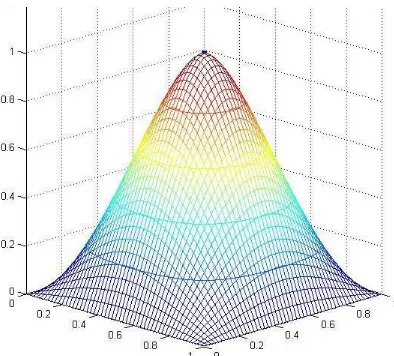
decreases, and we stop the iteration when the decrease is less than a treshold. Here is the picture of the surface, within a treshold of 10−4
[image:7.612.227.381.243.427.2].
Figure 1. The surface passing through (0.5,0.5,1) with minimum E1.5(u)
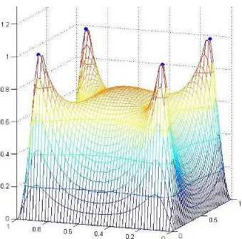
The following pictures are obtained for different order β and/or different points (xi, yj, cij).
[image:7.612.205.402.518.696.2]Figure 3. The surface passing through (0.5,0.25,0.25) and (0.5,0.75,1.25) with minimum curvature
Figure 4. A surface passing through four prescribed points with minimum E1.5(u)
Figure 5. Another surface passing through four prescribed points with minimum
[image:8.612.221.391.514.682.2]4. The Case 0≤β ≤1
Suppose that 0≤β ≤1 and we are trying to find a function uonS that minimizes the energyEβ(u) and satisfies u(0.5,0.5) = 1. The existence and uniqueness of such a function is guaranteed by Theorem 2.5, but as we shall see now the continuity is lost.
Recall that if v := [amn] is an element of V, then
∞ X
m,n=1
amnsin 0.5mπsin 0.5nπ = 0.
This implies that the only element that is orthogonal to V is u:= [sin 0.5mπsin 0.5nπ (m2+n2)β ] or
its multiples. But then we have
kuk2 = 2β1 + 2
5β + 91β + 132β +172β +251β +· · ·
>2β1 + 3.1 9β + 5.
1
25β +· · ·
=∞.
ThusV⊥
={0}orV =W, the whole space. This tells us that, starting from any initial approximation u0, we will end up with u = u0−projV(u0) = 0, that is, u(x, y) = 0
almost everywhere on S. Since we wish to keep the value 1 at (0.5,0.5), the function
u cannot be continuous on S. For instance, if we start from u0(x, y) = sinπxsinπy,
then we will end up with
u(x, y) =
1, (x, y) = (0.5,0.5),
0, otherwise.
This result is actually predictable in the case β = 0, that is, when we minimize the volume under the surface z = u(x, y), subject to the condition u(0, y) = u(1, y) =
u(x,0) =u(x,1) = 0 and u(0.5,0.5) = 1.
To sum up, to have a continuous solution to our minimization problem, the condition
β >1 is not only sufficient but also necessary.
Acknowledgement. H. Gunawan and L. Ambarwati are supported by ITB Research Grant No. 252/2009. The pictures are produced by using Matlab; we thank I. Sofyan and F. Pranolo for having translated our ideas into the codes.
References
[1] A.R. Alghofari,Problems in Analysis Related to Satellites, Ph.D. Thesis, The University of New South Wales, Sydney, 2005.
[2] R. Ardon, L.D. Cohen and A. Yezzi, “Fast surface segmentation guided by user input using implicit extension of minimal paths”,J. Math. Imaging Vision25 (2006), 289–305.
[3] K. Atkinson and W. Han, Theoretical Numerical Analysis: A Functional Analysis Framework, Springer-Verlag, New York, 2001.
[4] F. Benmansour and L.D. Cohen, “Fast object segmentation by growing minimal paths from a single point on 2D or 3D images”,J. Math. Imaging Vision33(2009), 209–221.
[6] H. Gunawan, F. Pranolo and E. Rusyaman, “An interpolation method that minimizes an energy integral of fractional order”,Proceedings of Asian Symposium on Computer Mathematics 2007
(published by Springer-Verlag in 2008).
[7] H.L. Langhaar,Energy Methods in Applied Mechanics(John Wiley & Sons, New York, 1962). [8] G.G. Lorentz,Approximation of Functions, AMS Chelsea Publishing, Providence, 1966. [9] C.R. Rao and M.B. Rao, Matrix Algebra and Its Applications to Statistics and Econometric,
World Scientific, Singapore, 1998.
[10] E.M. Stein,Singular Integrals and Differentiability Properties of Functions, Princeton University Press, Princeton, 1971.
[11] J. Wallner, “Existence of set-interpolating and energy-minimizing curves”, Comput. Aided Geom. Design21(2004), 883–892.
[12] W.L. Wan, T.F. Chan and B. Smith, “An energy-minimizing interpolation for robust multigrid methods”,SIAM J. Sci. Comput.21(1999/00), 1632–1649.
H. Gunawan: Analysis and Geometry Group, Faculty of Mathematics and Natural Sciences, Bandung Institute of Technology, Bandung, Indonesia.
E-mail: hgunawan@math.itb.ac.id
E. Rusyaman: Department of Mathematics, Padjadjaran University, Bandung, In-donesia.
E-mail: rusyaman@plasa.com
L. Ambarwati: Analysis and Geometry Group, Faculty of Mathematics and Natural Sciences, Bandung Institute of Technology, Bandung, Indonesia.