Financial Economics
Lecture 4
Stephen Kinsella
∗February 1, 2010
1
Introduction
In previous lectures, we looked at the market as a structure, and as a set of probabilistic concepts. This lecture and the one after it will concentrate on looking at the market from a physicist’s viewpoint. The seminal work in this area was done by MFM Osborne in the 1960’s1
It is important for us to look at the market from a physicist’s viewpoint because many of the tools and concepts we use in financial economics come originally from physics, so a change in perspective allows us to look at concepts anew. Moreover, the physicist is trained to look first at the data, then at the data some more, and once again, before coming to any conclusions about what underlying model may or may not be generating the data we see in reality.
It turns out that when you look at the data of a market for a while, you begin to ask yourself: what do markets do? Is supply and demand a good model of these interactions? Is the capital market a market for capital?
2
Is the capital market a market for capital?
The finance industry obviously has a vested interest in proclaiming the usefulness of the stock market to society: they will say the market creates wealth, it ensures liquidity, it raises capital for new ventures. Perhaps all of this is true. But what if the stock market is just legalised gambling, which has as side effects the three features I mentioned above? From this perspective things seem a little different.
One way to understand this question is to ask whether we can distinguish between ‘new’ capital, created by the market in a period, and ‘old’ capital, just being moved around. It should be obvious to you that there is almost no way to do this. We could look at total net investment over a period, the net change in stocks issued, or a number of other measures. Do you think these measures would give you the answer you seek? If so, why? If not, why not?
One effect the market does have on society is liquidity. The market produces liquidity, so that you, the buyer can move your money around from one product to another in the hope ofmaking some more money. From whom are you making it?
You should realise that a fertile way to explain the market is as a sort of competitive gambling. Ev-eryone wants to make money from someone else. Wealth is being moved around, mostly by noisy trading. Noisy trading is trading on poor or misguided information, perhaps rumours, rather than the mean-variance approach we’ll develop in later lectures.
Now let’s take a look at supply and demand, and reformulate it to have some bearing on the discussion of limit order markets I’d like to show you.
∗Department of Economics, University of Limerick, Ireland. Email[email protected].Webwww.stephenkinsella.net.
3
Supply and demand vs. reality
How are prices generated?
You should know the answer to this question from your lectures with Prof. Dineen and Dr. Lenihan. The interaction of supply and demand produces the price. There are, in any market, a set of suppliers, arranged in an schedule. There are a set of demanders, arranged in a schedule. These market participants enter a room somewhere and thrash out a price. After some time, the price they achieve is the equilibrium price, where buyers’ willingness to pay is equated with sellers’ willingness to sell.
We get a picture of this interaction in the form of decreasing demand curves, increasing supply curves, and a tried and trusted equilibrium point, just like figure 1 below.
Figure 1: Textbook supply and demand.
The plan is to tease out the implicit assumptions of this figure, to get a sense of where it can be changed to come into line with reality a bit more. Once we have done this little task, we will be in a situation where we can use the supply and demand model more effectively in our study of simple limit order markets.
3.1
A mathematical digression
From a physicist’s point of view, this picture of market exchange doesn’t work too well as a description of reality. This version of the supply and demand story is based on the works of Alfred Marshall, a famous Cambridge economist who developed the marginal theory of market equilibrium.
We’re going to mess around with the Supply and Demand graph you’re all familiar with, in order to make some points about the functioning of the market.
First, what does a market actually do? We’ve talked in previous lectures about the market working somehow to reduce risk, or to provide liquidity, or to transfer wealth, or to generate prices for previously unpriced attributes of products and services. But what if this is all wrong? What if the market is just a legalised form of gambling, a side effect of which is the extra liquidity we sometimes see in the markets? From this rather negative vantage point, what is the role of the market? How are prices generated? What does it mean for the textbook analyses of supply and demand? To answer these questions, we first need to start talking about what mathematicians mean when they talk about functions.
price at that time.
In mathematics, a function is a rule which maps an element of one set onto a corresponding element in another set. Start out with two sets, which are just two lists of objects. Now each set has some things in it, summarised by the functionalsX =xand Y=y. So, an element of a set,y, is related by the function to an element in the set,xby a rule, which is the function. If you pick an object from the setX, the functional relationship tells you uniquely which objectyin the setY xis associated to. We summarise this relationship by sayingy=f(x).
The language used here is the function ( a relationship) is defined over the domain, which is the setX, and the function itself, the y, is specified over the range of the set Y. This means there are very defined limits to the relationship between X and Y. This is so we can speak very precisely about their relationships. Please note that just because the function tells you whichxyou’ll get for eachy, in general, it does not follow that the opposite is true.
Example. The set of all TDs in the Dail, and the set of all voters. For each voter, there is a defined TD. So, for example, the element Stephen Kinsella in the set is associated with the TD Willie O’Dea. That is easy. So TD is a function of Voters. But Voters are not a function of TDs, because there is no unique voter for each TD. If you pick a TD, say Willie O’Dea, you do not automatically pick a unique voter.
Exercise 1 Set theory question A second example is the set of all mothers and the set of all children. Why?
3.2
Idealised vs. Actual supply and demand
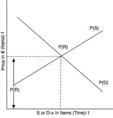
It is a mathematical convention that the vertical axis is used for plotting the function, or range set, and the horizontal axis the domain set. In the diagram above, we have 3 types of prices, P(S), the supply prices,P(D), the demand prices, and P(R), the prices you would see in the real world. Textbooks don’t show the differences between these three, which is a shame, because we have to be careful in determining the independent variables and the domain set. Getting these things wrong could cost us a lot of money, so beware.
The figure above has two interesting properties. First,P(D) andP(S) are definitely the functions. The figure implies you can go uniquely from any point onP(S) to any point onP(D). This is not necessarily true. In the figure above, the domain and range sets can exchange their roles: so if we haveP=P(D), then by inversion we can always getD=D(P). Second, the curves are continuous, so, at any point, the ordinate,
P, and the abcissa,D orS, is sharpley defined numerically, everywhere on each curve. What this mean is, the derivative can be taken at any point. We don’t live in a continous world though, but the functions above suppose we do. We need to take account of these issues to make a sensible model of an auction market and a limit order market after that.
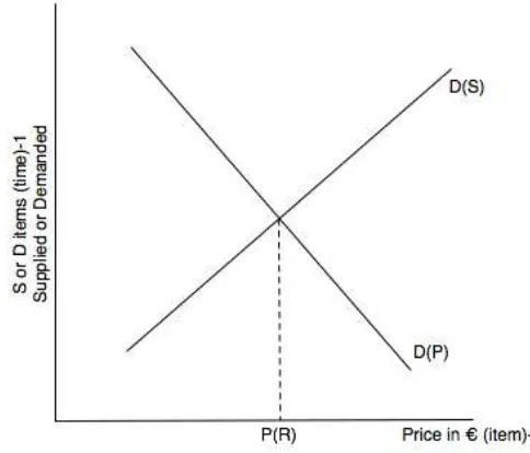
Let’s redraw the familiar supply and demand diagram to make some sense of them. Let’s keep D(p) sloping down, and D(S) sloping up, so they are increasing and decreasing functions of the price, which they were intended to be. Let’s plot supply and demand not as functions of quantity, as above, but as functions of price, as below.
Now, look at the figure below. We’ll discuss it in depth in the class.
3.3
How do economists get supply and demand curves?
You may have asked yourself the same question in your time as an undergraduate at UL: how do these guys actually find these curves? Well, to make the curves we see, we need a set of points in Price, Quantity space. To find out what this might look like, let’s consider an example.
Mrs. Ryan goes looking for a dress.
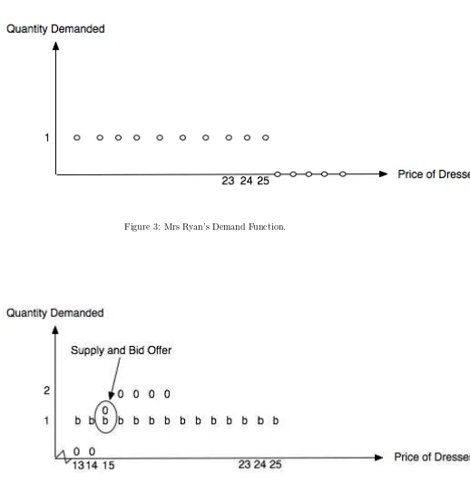
Mrs. Ryan would like to purchase a classy number for her night out. She is willing to pay 25 euros or less for it. Her demand function for this dress (of which she wants only 1), is given by figure 3.
Figure 2: Idealised supply and demand.
forever and a day. The demand function really is a function of five variables: price, which we graphed, longitude, latitude, and altitude, and time. We are, implicitly, holding these last four constant so we can make the graph shown in 3.
If she finds a shop that has the dress for 25 or less, then Mrs Ryan will happily buy it. Say she walks into a shop, and on the first floor finds two dresses (which fit her) for sale at 15 euros. The dresses are exactly what she was looking for.
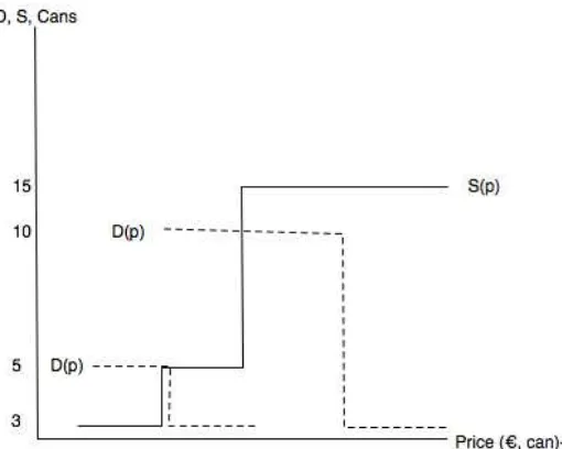
What does the interaction of the shop’s supply function, and Mrs. Ryan’s demand function, look like? It looks like figure 4.
Not that if the shop is not open, or if Mrs. Ryan is early or late, the supply function is zero, so far as she’s concerned. Also note that, following her transaction, the supply and demand curves change. Only one dress remains in the shop, and Mrs. Ryan’s willingness to pay for another dress exactly like that drops to zero.
Think about the asymmetry of information between Mrs. Ryan and the shop at this point. Mrs. Ryan knows the supply function of the shop: she can see the prices and the quantity supplied. Once she sees the price is less than her maximum willingness to pay, she slides her demand function back down to 15 (from 25), and there the supply and demand functions intersect.
Now let’s generalise what we see in the case of Mrs. Ryan’s example. A supply and demand diagram might look something like figure 5.
Now imagine Mrs. Ryan wants an haute couture dress. She goes into the Limerick branch of the Prada store, and sees one that fits. She likes it, but can’t see the price anywhere. The sales person simply tell her to write the price she is willing to pay for it, and if the shop owner agrees, then Mrs. Ryan has her sale. (Note the increase in the asymmetry of information here).
Now imagine Mrs. Ryan is told she can get any type of dress she wants. If she wants it, they’ve got it. She finds the dress, goes to buy it, but is stopped by a ‘broker’, who explains to her the way this shop works. He says “ You write what you’re willing to pay on a piece of paper, and I’ll go to the owner and find out what he’s willing to sell it for. Then if the prices overlap, I’ll decide what price will be satisfactory to you both.”
The seller decides to sell for 15, the broker makes 5, and Mrs Ryan walks out with a dress for 20, thinking she saved 5 euros.
Figure 3: Mrs Ryan’s Demand Function.
Figure 5: Interaction of hypothetical supply and demand.
was. 10. He knew Mrs. Ryan’s willingness to pay was 25. The seller did not. He could have asked her for more, but he didn’t. Why not? Perhaps he is honest, or perhaps his cut is regulated. Either way, all three parties win.
4
The limit order only interrupted market
A limit order to buy simply means you have to specify how much you want, and the most you are willing to pay for it, exactly like Mrs. Ryan. The limit order is a sort of demand function, in that it is a function of price, and it is discrete.
For example, if you want to buy 200 Apple shares at 50 euros a share , the demand function is a horizontal line of dots at 2 up to 50, and after that, it drops to zero, indicating you won’t pay more than 50 for Apple stocks.
A limit sell order is the opposite, and it exactly determines your supply function, as in the case of the department stores.
Placing all limit buy orders together at some point in time and space determines a limit order only interrupted market where buy and sell orders are matched for execution.
The process always gives a highest bid, a lowest offer, a quote, or a transaction at a given price.
The process is totally mechanical: once the buyers and sellers input their maximum bids for sale or purchase, the broker matches up each side of the market, distributes sales (if they occur), and purchases (if they occur), and takes her cut.
Let’s look at an example.
4.1
Example
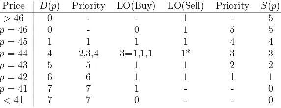
Here we’ll only use integers for trades, no 1/8 or 1 cent rules. What is the match point price?
Price D(p) Priority LO(Buy) LO(Sell) Priority S(p)
Table 1: Limit Order example. LO(Buy) is a limit order to buy, similarly for LO(Sell). Source: Osborne, (1977), pg. 42.
Table 2: Limit Order example. LO(Buy) is a limit order to buy, similarly for LO(Sell). Source: Osborne, (1977), pg. 42.
5
Exercises
Exercise 2 Limit Order 1Solve this limit order market with differing order sizes. Solve for the match point price. What does this tell you about buying in bulk?
Do you see the difference between assuming a line when in reality it is a line of closely spaced dots?
Exercise 3 Limit Orders with many products (From Osborne [1965, pg. 91].)
Take the data of table 4.1 and double every order. Now add at P = 1000first 1, then 2, then 3, then 4, etc. The idea is thatp= 1000represents a positive infinity for limit orders. Use the following rule to make out strike prices: take the mean of the possible highest and lowest match point price, to find the executed (strike) prices, and the transaction sizes. How many really big price jumps at p= 1000 before you settle down top= 1000with an order size of 10?
6
Some real world context
Many financial markets around the world, including the Paris, Stockholm, Shanghai, Tokyo, and Toronto stock exchanges, are organized as limit order books.
the market sorts buyers and sellers by willingness to buy or sell, applies an ambuigity rule to the nearest unit, and notify those customers if a transaction was or was not made. When orders are of the same size, one applies a ‘first come first served’ priority rule on buyers, then sellers.
A limit order only market assures that all market participants have the same information.
The role of a dealer in securities markets is to provide liquidity on the exchange by quoting bid and ask prices at which he is willing to buy and sell a specific quantity of assets. Traditionally, this role has been filled by market-maker or specialist firms. In recent years, with the growth of electronic exchanges such as Nasdaq’s inet, anyone willing to submit limit orders in the system can effectively play the role of a dealer. Indeed, the availability of high frequency data on the limit order book (see www.inetats.com) ensures a fair playing field where various agents can post limit orders at the prices they choose.
Definition 1 (Limit Order) A limit order is an instruction to trade a specific quantity of an asset at a specified price, or a better price. The order is an ex-ante precommitment(t, j, x, p)made on a datetto trade up to a given amount x of an asset j at a prespecified limit price p. The order is in force until filled or cancelled, so unfilled orders accumulate in an limit order book Kyle [1989].
Definition 2 (Limit Order Book) The limit order book is characterised by a discrete set of prices at which traders may submit orders. The tick size, or distance, between any consecutive prices, is normalised to one. A backlog is associated with each price at any time. The backlog is the depth of the market at that price. The Limit order book is the vector of outstanding orders at any point. Given a limit order book, the bid price or quote is determined by the highest price at which a limit buy order exists, and the ask price or quote is the lowest price at which there is a limit sell order on the book. The book can, of course, be empty—then no market exists at all.
Limit orders are executed according to time and price priority, meaning orders submitted earlier are placed further ahead in the queue. Buy orders at higher prices and sell orders at lower prices get priority. An order will execute if no other orders have priority, and a trader arrives who wants to buy at some price. All trades execute instantly at the ask, and that order becomes themarket order at this point.
Limit orders differ from standard market orders, which are requests to trade immediately at the best available price in the market. In a limit order setting the order execution is always filled at the limit price set by the buyer or seller. In limit orders, price priority holds, which means the limit orders offering better terms of trade (buyers buying higher, sellers selling lower) execute ahead of limit orders at worse prices. Time priority can also hold, where at each pricep, older limit orders are executed ahead of newer ones in a queuing system which thus rewards first movers who give up liquid positions to allow the LOOM to work more effectively. The price and time priorities may be taken together to define a probability distribution over execution timing. The notion of equilibrium in limit order markets is different to other continuously clearing markets, because buyers arrive and trade asynchronously in a limit order market, so there is no unique market-wide ‘market-clearing’ price, except in degenerate cases. Rather, there is a sequence of bilateral transaction prices at which endogenously matched pairs of investors choose to trade over time.
References
A. Kyle. Informed speculation with imperfect competition. Review of Economic Studies, 56(1):317, 355 1989.
M.F.M. Osborne. Dynamics of stock trading. Econometrica, 33(1):88–113, 1965.