DOI: 10.12928/TELKOMNIKA.v13i4.1895 1214
Routing Algorithm Based on Area Division
Management of Node in Wireless Sensor Networks
Gao Wei1,*, Song Yan2, Shuping Fan1 1
Institute of Technology, Mudanjiang Normal University, Mudanjiang157011, Heilongjiang, China 2
Department of Scientific Research, Mudanjiang Normal University, Mudanjiang 157011, Heilongjiang, China
e-mail: [email protected]
Abstract
In order to reduce the communication overhead among sensor nodes, a routing algorithm is proposed based on zoning management nodes. The algorithm defines the calculation method of the network partition radius after nodes deployment, and divides monitored area according to the radius meanwhile layouts one management node in each partition. Then nodes’ communication cost is calculated based on the distance among nodes as well as nodes’ energy, and finishes the selection of routing nodes based on the cost. Finally, using the Matlab simulation environment, the parameters impacting the optimal partition radius are discussed, and the proposed routing algorithm is compared with existing algorithms. Theoretical analysis and experimental results show that the proposed algorithm is more balanced on nodes energy consumption. The algorithm reduces network traffic overhead while extends the lifetime of the network.
Keywords: Wireless Sensor Network, Management Nodes, Routing Algorithm, Communication Overhead, Partition
Copyright © 2015 Universitas Ahmad Dahlan. All rights reserved.
1. Introduction
Wireless Sensor Networks (WSN) is generally made up of thousands of self-organized sensor nodes which are very small. As sensor node can also sense and process information together with communicating with other nodes, people design wireless sensor network to monitor various situations or events, transmitting the node data to terminal users. However, although there is limited strength of sensor node in practical application and WSN will save strength as much as possible by applying great network topology and best routing strategy. But because of the difference between traditional network and Ad hoc network, route in WSN are paid more and more attention [1, 2].
Depending on the event-driven nature of WSN, the main function of sensor node in different applications is to forward the perception data from target zone to base station. Therefore, designing efficient routing algorithm to build high quality path is one of most important issues in WSN [3, 4]. For the inherent features of WSN, routing in WSN is a challenging problem. In recent years, scholars home and abroad proposed that there are mainly two routing algorithms [5, 6, 7]: single path routing algorithm and multipath routing algorithm. The former is easy to be realized and good in expansibility, but has high network energy consumption, and thus it cannot meet the requirements of resource-constrained WSN. Multipath routing algorithm is a technology that can be used to substitute routing technology. Through the paths it chooses, the data can be transmitted from the source to the target. Compared with single path routing, low delays, load balancing and high link quality of multipath routing technology has significantly improved WSN performance and attracted more and more attention.
network partition, in the end give routing process of the node. Through the theoretical analysis and simulation experiment, the result shows that the network expansibility of the proposed routing algorithm is good, while reducing energy consumption of node and balancing node load, lifetime of network is delayed.
2. Research Method
A lot of routing policy is raised in recent years, in order to provide the use ratio of network energy. Apply the traditional routing algorithm CR [3]. When node detects the events, it will broadcast them to all the nodes (these nodes are called neighboring nodes) within the range of telecommunication. The neighboring nodes will also broadcast the information to other nodes. The process will be going until the event reaches base station (BS), which results in over consumption of node strength in network and adds the conflict in wireless transmission. In order to improve the utilization of network strength, many routing strategies are put forward in recent years [4-12]. LEACH [4], whose execution process is periodical, is the typical routing algorithm in WSN. Every circulation consists of stage of cluster establishment and stage of data telecommunication. The routing algorithm divides network into many clusters in network by randomly creating cluster head, from which it sends, receives and combines data to reduce the strength consumption of common nodes. But in the process of cluster head directly transmitting data, LEACH algorithm does not consider the actual physical distance from node to base station, which leads to node consumption’s rapid increasing along with bigger distance from base station. Therefore, this algorithm does not fit in WSN’s large-scale environment. The scholars later come up with the improved algorithm like LEACH-TE [5] and LEACH-CE[6] against the disadvantages of LEACH. In choosing cluster head, the former considers remained strength of node and average strength in the whole network. The latter introduces the concept of backup cluster head. Both of the algorithms calculate the best cluster numbers from the principle of least strength. Compared with LEACH, these two algorithms are better. Eight people including Wang Kunchi [7] and Duan Wenfang [8] come up with the routing algorithm based on“minimum hop”. The basic idea of this algorithm is to establish “minimum hop”and timely add new nodes by sending messages with each other among the nodes. The two algorithms optimize the process of data transmission and use ACK as well as message cache mechanism. In addition,the document [8] puts forward Hello packet jumping mechanism and provides the maintenance process of route. RDSR [9] puts forward another kind of routing idea, which divides the network into several areas based on the relative direction of transferring data. Then the node will randomly select relay nodes in all areas according to the relative position distance from base station. The node route process of using this algorithm is easy, but when the divided areas are relatively large in network, routing circle will be created in network because of node’s random selection. Document [10] and [11] put forward routing path to find node by creating routing table for shortcomings of RDSR. Document[12] put forward ERIDSR algorithm, which introduces “minimum hop” and adds the factors of telecommunication distance. In order to further save the strength of node and improve the routing efficiency of network, a kind of new routing algorithm is created based on area division management of node.
3. Routing Algorithm Based on Area Division Management of Node
Similar to LEACH algorithm, the execution process of routing algorithm is periodical, but every cycle is divided into three stages: setting network, dividing area and transferring data.
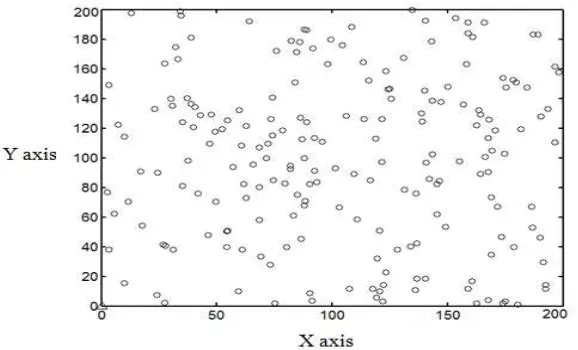
3.1. Production of Network Topology
Figure 1. Structure of network arrangement.
3.2. Area Division Process of Network 3.2.1. Calculation of Subarea Semi-Diameter
It is assumed that sensor node in network can dynamically sense the remained strength and position itself as well as calculate the distance from base station or other nodes by using
I-ERIDSRalgorithm. The i subarea semi-diameter in network is Ri(1 i tt i, Z), of which tt represents the total number of subarea semi-diameter. The calculation formula is as Equation (1).
In Equation (1), d1 is the telecommunication threshold and it is set that all nodes in the range of d1away from node i (1 i n) are the neighboring nodes. The n is the number of common sensor node in network. In form network the unified parameter c1 and c2 are two important ones in establishing subarea structure by setting different values in practical use to flexibly change the division of network area. Parameter c1is used to decide the size of semi-diameter R1 in the first subarea, which indirectly affects the size of semi-semi-diameter in other areas and finally will affect the area in all subareas. Parameter c2 affects the semi-diameter value of other subareas except for R1, which makes the values of parameter c1and c2in R1as 0.2 and 3. The value of Rican be seen in Figure 2. Value of minimum subarea semi-diameter in network depends on the furthest node from base station in network.
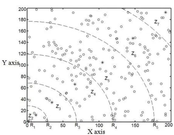
Figure 2. Topology structure of network dividing area
3.2.2. Division of Network Area
Base station, which will be regarded as center in network, will calculate the network subarea semi-diameter. Riis the semi-diameter to produce many virtual circles. In order to make it convenient for instruction, it is shown in the dotted line of Figure 2 that base station will divide network into several fan shape areas according to these circles. After dividing areas, base station will broadcast information to node of arrangement area. When node is received, it will calculate the area number itself according to the distance from base station. The process of network dividing area and calculation process of node area number are as followed:
(1) The broadcasting information packet HELLO(IDi,(N(i).xd,N(i).yd),d1)of node i in network includes the identifier IDi with node i, coordinate(N(i).xd,N(i).yd) of node i and telecommunication threshold d1, After another node j receives packets, it will calculate the absolute value dijaccording to the distance from node i. Ifdij d1, node i will regard node j as neighboring one and store it in routing table.
(2) Base station regards R1as telecommunication semi-diameter and sends the packet Message (n+1,(N(n+1).xd,N(n+1).yd ),Ri), identifier with base station in message, base station coordinate and calculation formula of subarea semi-diameter. After node i receives message in area 1, it will calculate the absolute value of distance from base station and store Ri according to base station coordinate. Later node i will send data packet Message1 (i,n+1,(N(n+1).xd,N(n+1).yd ),d1) to the neighboring node.
(3) After neighboring node j in node i is received, it will calculate the absolute value of distance from base station according to the message, change the node identifier i to j in Message1 and later will forward to other neighboring nodes.
(4) Repeat step (3) until all nodes have calculated the distance from base station.
(5) Base station compares with the area semi-diameter according to the distance absolute value from the furthest node. If Rt1MAX_DisRtbase station will gain the total number t of divided area in network.
(6) Node i will calculate the area number N(i).Z itself according to the absolute value of distance from base station. The calculation formula is:
1?1 IfdiBSR1, then N(i).Z=1;
2? 2 Otherwise,ifRi1diBS Ri, (i2),then N(i).Z=i.
horizontal axis represents subarea semi-diameter. Base station will arrange a management node in every area after dividing areas. As node “*”is shown in figure, this kind of node position in area is fixed and the strength is out of limit.
3.3. Routing Process of Node
In order to further improve the routing efficiency of node, the algorithm (recorded as I-ERIDSR) fully considers the subarea number and strength of node, distance from node to management node or base station in selecting routing node, which node i will choose from all neighboring nodes j(1 j n j, i) according to the size of telecommunication cost. The telecommunication cost N(j).cost of node j is defined as:
2 2
It is not hard to find from formula (3) that the bigger the strength of node j, the nearer distance from management node or bigger probability to forward data as the next node. In order to ensure the effectiveness of algorithm, the nodes near base station will directly send data to the station. The process of node i i( n 1) in selecting route is concluded below:
The 1-4 line of the algorithm above is an initial process of parameter, of which MNnum represents the numbers of management node in network. As the definition of identifier in base
---
12 ?12 COMPUTE N(tempHeads(j)).cost
13 ?13 end
14 ?14if(N(tempHeads(j)).Z<N(i).Z)
15 ?15 if(N(tempHeads(j)).cost ==mincost)
16 ?16 N(i).nexthop=tempHeads(j) ;
17 ?17 end if
18 ?18 else if(N(tempHeads(j)).Z==N(i).Z&& N(i).nexthop==0)
19 ?19if(N(tempHeads(j)).cost ==mincost1)
20 ? 20 N(i).nexthop=tempHeads(j) ;
21? 21 end if
22 ? 22 else if(N(tempHeads(j)).Z>N(i).Z&& N(i).nexthop==0)
station is n+1, the identifier of management node will begin from n+2. N(i). flag_multiHop is used to indicate if node i applies way of multi-jumping to transfer data. Initiative value of 1 refers to use way of multi-jumping and N(i).nexthop is used to store the identifier of next jumping route in node i with initiative value of 0; the5-9 line of the algorithm is used to judge the area number size of nodei(1 i n).If area number equals 1, node i does not need to forward data by other nodes but to directly send data to base station. At this time, the multi-jumping identifier variable of node i will be set as 0; the 10-27 line is used to use way of multi-jumping to send data of node i routing process, of which the 10-13line is used to calculate all telecommunication cost N(tempHeads(j)).cost of neighboring node in node i. The 14-27 line uses multi-jumping routing strategy: at first node i will choose the minimum neighboring node j as the next jumping route in all neighboring nodes where area number is the smallest. If there is no such routing node in the 14-17 line of the algorithm, node i will respectively select according to area number with equal and bigger sequence from the neighboring node in corresponding areas based on the principle of minimum telecommunication cost which can be seen at 18-26 line; the 29-30 line is used to define routing node of management node in section 1 as base station and set the multi-jumping identifier of management node as 0; the 31-35 line is used to define the routing node of other management nodes except for section 1. The next jumping in this kind of node is smaller than the management node of area number. It is not hard to see from the routing node selection algorithm defined in this text that node will prefer to select the nearer area neighboring node from base station as relay node. In this way, it will reduce the telecommunication cost of node and save the strength of node, which is crucial to wireless sensor with limited strength.
4.Simulation Experiment
4.1.Experiment Environment and Parameter Setting
Imitate operating environment of network in the Matlab simulation platform by setting experiment parameter. It is defined the best calculation formula of subarea semi-diameter in routing algorithm(I-ERIDSR) of this text according to the experiment result. We will also make comparative analysis between I-ERIDSRalgorithm and RDSR, ERIDSRalgorithm. It is assumed in experiment that there are 200 common sensor node randomly scattered in the two-dimensional area of 200m*200 m in which the initial strength of node is 0.5J and size of data packet is 400bits.
The experiment value of telecommunication threshold d1 is 30m. Part of other variable value in experiment is referred to document [13].
4.2. Experiment Result and Theory Analysis
4.2.1.Certainty of Parameter in Subarea Semi-Diameter Formula
Figure 3. Network consumption when parameter c1has different values
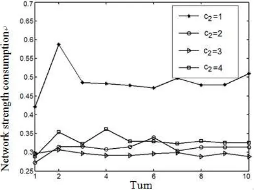
Figure 4 provides four different values of c2=1,2,3,4 when c1=0.2 the strength consumption trend of all nodes in every turn of network. The experiment result indicates that when c2is valued between 1 and 3, the whole consumption of node will gradually reduce in every turn of network. This is because when c2is valued too small (c2=1 or 2) and divided areas in network are relatively many, the area of small number will be lower and the nodes are fewer too. But these nodes often need to forward the data of bigger area number which are sent by node. As a result, the node consumption will be more and will die early. The node consumption of all areas are not balanced, which will make the whole performance of network go down. It also can be seen from Figure 4 that when c2 is valued more like 4, the network consumption is increasing. This is because when c2is valued more, the subarea number in network is too little and number of management node is not much and the nodes of all areas except section 1 send data, it needs not many management nodes to send, which will result in the forwarding circulation and more consumption in network. Therefore, the best value of c2 is 3 in the experiment environment of routing algorithm provided in this text.
4.2.2. Comparison of Strength Consumption
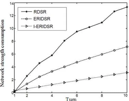
In Figure 5 we make comparison of the node consumption in network when the three algorithms of RDSR, ERIDSR and I-ERIDSR operate i(i=1,2,…10) turns. Simulation experiment has been done for 10 turns and the node in every turn transfer only one data. It is not hard to see from Figure 5 that the consumption of RDSR algorithm is the biggest with the increasing of turns and the corresponding strength curve is not smooth. The node strength other two algorithms keeps steady growth and the consumption of routing algorithm I-ERIDSR provided in this text is the smallest. This is because in the routing process of using RDSR algorithm node will randomly select node as relay nodes in all subareas according to area numbers which can not ensure the optimization of node. This will make some nodes transfer data in long distance and consume big node strength. In addition, if node arrangement in RDSR algorithm is in the subarea with bigger area number and far away from management node, node will produce routing circle in this area which will make the node run out of strength and die early. Thus, using the whole network of RDSR algorithm will have big algorithm and imbalanced node consumption. There are three factors among jumping number, area number and node in the process of choosing relay node in ERIDSR algorithm. Compared with RDSR algorithm, the whole consumption of ERIDSR algorithm will be lower; and I-ERIDSR algorithm divides area of network through experiment to define the best calculation formula of subarea semi-diameter in order to realize the goal of reducing telecommunication consumption of node. Moreover, this algorithm considers the area number and telecommunication cost in the process of node route. The calculation of telecommunication cost considers two factors of strength and distance, which makes stronger direction to destination node in time of sending node data. As a result, compared with RDSR and ERIDSR algorithm, the whole consumption of I-ERIDSR algorithm is lower.
Figure 5. Comparison of Network Consumption
4.2.3. Comparison of Network Life
In order to test the surviving time of network, we make comparison of node death after using three algorithms of network to operate 50 turns. As I-ERIDSR algorithm has not appeared death node in the first 25 turns, the comparison of node death number in three algorithms will begin from the twenty-sixth turn. Experiment result is seen at Figure 6, from which it can be seen that after network operates 26 turns, we will use RDSR algorithm with more than 50 node death numbers. The node death number of ERIDSR algorithm is about 30, but in the same turn the node death number of I-ERIDSR algorithm which is obviously smaller than RDSR, ERIDSR algorithm. With the growth of each algorithm’s operating turn, the node death number of I-ERIDSR algorithm in network increases slower than RDSR, I-ERIDSR algorithm. This is because the consumption of I-ERIDSR algorithm is more balanced and obviously less than RDSR,
ERIDSR algorithm in the condition that three algorithms have the same common experiment parameter. Therefore, the death node number of this algorithm in network is less with longer surviving time of network.
Figure 6. Comparison of death node number
4.2.4. Comparison of Network Extension
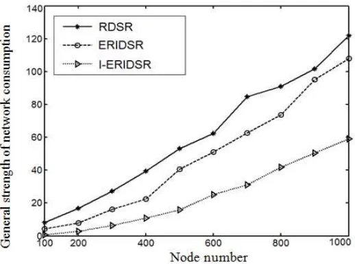
In Figure 7 we will use the node number of three algorithms in network when n=100,200,…1000 and make comparison of network strength consumption. The experiment has been done ten times. Each algorithm operates 10 turns in every experiment. We make comparison of the general strength consumed in ten turns. It is not hard to see from Figure 7 the whole network strength consumption of three algorithms tend to increase with the growth of node numbers. And in the condition that node numbers are the same in network, the consumed strength of I-ERIDSR algorithm is obviously lower than RDSR, ERIDSR algorithm, which indicates that I-ERIDSR algorithm network has good extension. This algorithm fits for WSN of large-scale node.
4.2.5. Comparison of Load Balance
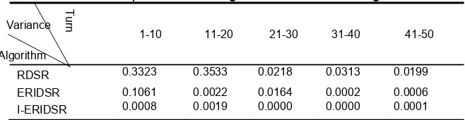
In order to test the node load balance of three algorithms in network, we will compare the strength variance of node in network in the condition that three algorithms have the same common experiment parameter. The approximate value of variance is rounded to four decimal places. Every algorithm experiment has been done 50 turns and we analyze the variance of general strength of network consumption on every turn of each algorithm namely in 1-10,11-20,…41-50 turn. Experiment result is seen at Table 1 and we can see from the data in Table 1 by using RDSR algorithm the consumed strength of node in every network turn varies because of random selection of routing node. As a result, variance value is larger while ERIDSR algorithm has stronger direction in the process of node sending data to management node or database. Therefore, compared with RDSR algorithm, the consumed strength in each turn of network node will be relatively balanced with small variance. Compared with the first two algorithms, variance of I-ERIDSR algorithm has little fluctuation. This is because in the process of using node routing algorithm in this text, the remained strength of routing node is considered which will balance node load and makes node strength consumption in every turn of network more stable.
Table 1. Comparison of strength variance in three algorithms
1-10 11-20 21-30 31-40 41-50
RDSR 0.3323 0.3533 0.0218 0.0313 0.0199
ERIDSR 0.1061 0.0022 0.0164 0.0002 0.0006
I-ERIDSR 0.0008 0.0019 0.0000 0.0000 0.0001
5. Conclusion
For the problem about big strength consumption of routing algorithm, we come up with a kind of routing algorithm I-ERIDSR based on area division management node. This algorithm consists of three stages: setting network, dividing area and transferring data. I-ERIDSR algorithm will divide network into several subareas according to subarea semi-diameter. Later a management node will be produced in every subarea. In the process of node sending data node strength and telecommunication distance among nodes are considered which makes the algorithm in this text have good performance in the whole. At last we make comparison between I-ERIDSR algorithm and existing routing algorithm. The result indicates the node of routing algorithm has balanced load, which fits for WSN of large-scale node. This algorithm reduces node strength consumption and extends the network life at the same time.
Acknowledgements
This work was supported by Hei Longjiang natural science foundation (QC2013C067); Technology Foundationof Mu Danjiang Normal University (QG2014003); Open foundation project of Hei Longjiang Intelligence education and information engineering key laboratory (SEIE2013-05).
References
[1] Samra B, Mohammed B. A Novel strength Efficient and Lifetime Maximization Routing Protocol in Wireless Sensor Networks. Wireless Personal Communications. 2013; 72(2): 1333-1349.
[2] Radi M, Dezfouli B, Abu Bakar K & Lee M. Multipath routing in wireless sensor networks: Survey and research challenges. Journal of Sensors. 2012; 12(1): 650–685.
[3] Liu Y, Xiong, N, Zhao Y, Vasilakos AT, Gao J & Jia Y. Multi-layer clustering routing algorithm for wireless vehicular sensor networks. IET Communications. 2010; 4(7): 810–816.
[4] Marjan R, Behnam D, Kamalrulnizam AB, et.al. IM2PR: interference-minimized multipath routing protocol for wireless sensor networks. Wireless Network. 2014; 20(7): 1807–1823
[5] Younis O, Fahmy S. Heed: A hybrid, energy-efficient, distributed clustering approach for ad-hoc sensor networks. IEEE Transactions on Mobile Computing. 2004; 3(4): 660-669
Variance
Algorithm
[6] Sha MK, Gehlot J, & Greve R. Multipath routing techniques in wireless sensor networks: A survey. Wireless Personal Communications Journal. 2012; 70(2): 807-809.
[7] Intanagonwiwat C, Govindan R, Estrin D, Heidemann J & Silvia F. Directed diffusion for wireless sensor networking. IEEE/ACM Transactions on Networking. 2003; 11(1): 2–16.
[8] Al Karaki N, Kamal AE. Routing techniques in Wireless Sensor Networks: A Survey. IEEE Wireless Communications. 2004; 11(6): 6-28.
[9] Babak Namazi, Karim Faez. Energy-Efficient Multi-SPEED Routing Protocol for Wireless Sensor Networks. International Journal of Information and Network Security (IJINS). 2013; 3(2): 246-253. [10] Widhi Yahya, Achmad Basuki, Jehn Ruey Jiang. The Extended Dijkstra’s-based Load Balancing for
Open Flow Network. International Journal of Electrical and Computer Engineering (IJECE). 2015; 5(2): 289-296.
[11] Mark McDermott. Cognitive Sensor Platform. International Journal of Electrical and Computer Engineering (IJECE). 2014; 4(4): 520-531.
[12] Oh H, Bahn H & Chae KJ. An energy-efficient sensor routing scheme for home automation networks. IEEE Transactions on Consumer Electronics. 2005; 51(3): 836–839.
[13] OhH & Chae K. An energy-efficient sensor routing with low latency, scalability in wireless sensor networks. International Journal of Smart Home. 2007; 1(2): 71-76.