S
HORT
R
AINFALL
D
URATION
E
VALUATION IN
D
ESIGN
S
TORMS
D
EVELOPMENT
E
VALUASID
URASIH
UJANP
ENDEKD
ALAMP
ENGEMBANGANP
ERANCANGANB
ADAIMasimin 1) and Sobri Harun 2)
1) Department of Civil Engineering, Syiah Kuala University, Banda Aceh, Indonesia 23111, masimin@plasa.com 2)
Faculty of Civil Engineering, Universiti Teknologi Malaysia, 81300 Skudai, Johor Bahru, Malaysia.
ABSTRACT
A 5-minute incremental rainfall data taken from 5 stations distributed in Johor southwest region was analyzed to study an inten-sity-duration-frequency (IDF) related to design storm development. The study includes a regional rainfall analysis, determination of probability distribution, estimation parameter and quantiles of the distribution, development of IDF, and the comparison study for IDF estimates based on daily rainfall. In the study, the duration pattern is set to 15-, 30-minute, 1-, 2-, 4-, 8-, 16- hour, and 1-day. An X10- test is used for regional analysis to define homogeneous region and probability weighted moments (PWM) is used to do a frequency analysis. To see the presence of trends, the Kendall’s method is applied. It is found that the region is passed the tests to be the homogeneous region. Based on frequency analysis, the data tends to follow the generalized extreme value (GEV) and generalized logistic (GLOG) distribution. In regression analysis, the IDF-curve for return period of 2-, 5-, 10-, 20-, 50-, 100-, 200-, and 500-year tends to follow a power relationship. The IDF family curves calculated based on daily data gives over estimates about 10% compared to those of calculated based on the 5-minute incremental rainfall data.
Keywords: regional homogeneity, design storms, frequency analysis
ABSTRAKSI
Data hujan tiap 5 menit yang diambil dari 5 stasiun yang tersebar di wilayah barat daya Johor dianalisis untuk mem-pelajari intensitas-dirasi-frekuensi (IDF) yang berhubungan dengan pengembangan perancangan badai. Penelitian ini mencakup analisis hujan regional, penentuan distribusi probabilitas, estimasi parameter dan quantil distribusi, pe-ngembangan IDF, dan studi perbandingan untuk estimasi IDF berdasarkan hujan harian. Dalam penenlitian ini pola durasi diatur dalam 15-, 30-menit, 1-, 2-, 4-, 8-, 16-jam, dan 1-hari. Pengujian X10 digunakan untuk analsisi regio-nal untuk menentukan keseragaman regional dan probabilitas berat momen (PWM) digunakan untuk nanlisis fre-kuensi. Untuk melihat munculnya tren, metoda Kendall digunakan. Hasil analisis menunjukkan bahwa wilayah yang diteliti adalah wilayahyang seragam. Berdasarkan analisis frekuensi, data cenderung mengikuti nilai akstrim yang u-mum (GEV) dan distribusi logistik umum (GLOG). Pada analisis regresi, kurva IDF pada periode 2-, 5-, 10-, 20-, 50-,100-, 200-, dan 500-tahun cenderung mengukuti persamaan power. Kurva famili IDF berdasarkan data harian memberikan over estimasi sekitar 10% dibandingkan dengan data yang dihitung berdasarkan data hujan tiap 5 menit.
Kata-kata Kunci : Keseragaman wilayah, perancangan badai, analisis frekuensi
INTRODUCTION
Estimation of design storms is an unrest topic in statistical hydrology that needed in a broad spectrum in civil works espe-cially for an urban drainage design. One type of design storms development is classified as frequency based storm that the me-thod is based on statistical frequency analysis (Viessman and Lewis, 2003). Small size project with low hazard level is com-monly using this method with return period is less than 100 years. This study covers a topic of design storms with a case study area of southwest of Johor, Malaysia. The study includes a regional rainfall analysis, determination of probability distributi-on, estimation parameter and quantiles of the distributidistributi-on, deve-lopment of IDF, and the comparison study for IDF estimates ba-sed on daily rainfall data propoba-sed by Mononobe (Sosrodarsono and Takeda, 1980).
A rational method is a simple formula and widely used in design storms that the flow rate (Q) is a function of runoff coe-fficient (C), intensity (I), and area (A). Two variables C and A are the physical measures and variable I is a hydrological condition at the region. The value of intensity (I) is based on rainfall duration that equals or greater than time of concentration (tc). Design storm is mostly applied to short rainfall durations that the availability of short incremental rainfall data becomes problem because most of rainfall stations only give the data based on daily data bases. Rain-fall intensity prediction based on daily rainfall data was proposed and called as Mononobe method with the relation as in equation (1).
3 / 2
24
24
⎟⎟⎠
⎞
⎜⎜⎝
⎛
=
c T
t
R
I
(1)where, I = rainfall intensity (mm/hour); RT = daily rainfall for the
return period of T years; and tc = rainfall duration equal to its time of concentration (minutes). Although the rational method is very popular and widely used in defining the peak flow rate for urban drainage project, it has limitation for its coverage area. The method is suitable for the coverage area of less than 600 acres and for the coverage areas of urban drainage are greater than 600 acres, the hydrograph analysis is warranted (Viessman and Lewis, 2003).
Daud et al. (2002) studied of extreme rainfall process in Peninsular Malaysia and they found that the GEV was the most suitable distribution to be applied for annual maxima rainfall data in Peninsula Malaysia. The regional study for the state of Selangor using long duration rainfall data, it was found that the region of was determined as a homogeneous region and the sui-table statistical distributions were GEV and GLOG distributions (Masimin and Harun, 2006). There is no information yet for the study of design storms using short duration rainfall data in the region including for Johor. Adamowski and Bougadis (2003) stu-died about IDF using rainfall data in Canada and they found that the presence trends in short rainfall duration was significant in design storms.
comparison of IDF family curves defined based on daily rainfall data records to the those of first objective.
DATA AVAILABILITY AND PRELIMINARY ANALYSIS
Five rainfall stations in Johor provide a 5-minute incre-menttal rainfall for 25 years duration of record (1980-2004). Those five stations are Sta.1437116, 1534002, 15411139, 1636001, and 1732004. The first step in the study is to define an annual maxima rainfall depth based on the duration pattern. The ‘block method’ is used for data extraction that the block is defined based on duration pattern, so that it is not an event based but time based analysis. The reason of using the time base analysis is that a short duration rainfall is a ‘cloud burst’ and long duration rainfall is a multiple storms (Sveinsson et al., 2002). The event based analysis will give a small magnitude compared to those of time base data.
A preliminary data analysis is conducted by doing some sta-tistical tests included the independence and stationarity test and spatial correlation samples. The test for independence and station-nary is executed using equation (2) to (5) called the Wald-Wolfowitz testing method (WW-test) to test for the inde-pendence of a data set and to test for the existence of trend on it (Rao and Hamed, 2000). The WW-test showed that all the data set were passed to be independent as the statistical results were shown in Table 1.
u
=
(
R
−
R
)
/(var(
R
))
1/2 (2)
∑
=
+
=
+N
i
x
x
x
x
R
i i i N1
1(3)
R
=
(
s
12−
s
2)
/(
N
−
1
)
(4)))
2
)(
1
/((
)
2
4
4
(
)
1
/(
)
(
)
(
var
4 2 2 3 1 2 2 1 4 1
2 4
2 2
−
−
−
+
+
−
+
−
−
−
=
N
N
s
s
s
s
s
s
s
R
N
s
s
R
(5)
where u, R,
R
= the statistical test parameters;s
r=
Nm
r'
and' r
m
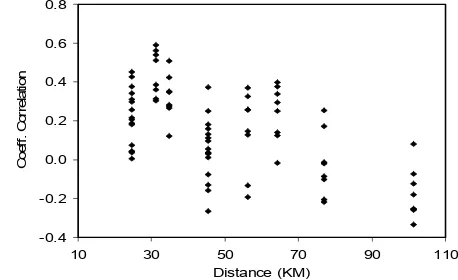
is the rth moment of the sample about the origin.The spatial sample correlation was used to examine the co-rrelation of every pairs observed point data sets that was sepa-rated by some distances (Kottegoda & Rosso, 1997; Berndtsson & Niemczynowics, 1986). The test was executed using equation (6) and it is about 80 tests are executed applied to the eight durations pattern for data sets. The results are plotted as in Fig.1.
∑
∑
∑
= =
=
+
−
+
−
+
−
+
−
=
Ni
N
i i i
N
i
i i
h
u
m
h
u
z
u
m
z
h
u
m
h
u
z
u
m
u
z
h
r
1 1
2 / 1 2 2
1
}
)]
(
ˆ
)
(
[
)]
(
ˆ
[
{
))
(
ˆ
)
(
)][
(
ˆ
)
(
[
)
(
(6)where r(h) = sample correlation;
m
ˆ
(
u
)
andm
ˆ
(
u
+
h
)
are the sample means of the observations at the two points.Fig.1 shows some information that some pairs of data points for a shorter distance (20-50 Km) give correlation values about zero and some data points for a long distance (70-100 Km) give correlation with greater values. Examining the loca-tion of the staloca-tions, the distance from the sea would be the signi-ficance parameter in partitioning the region to homogeneous sub regions. It is agree to the study of regional homogeneity using
SPATIAL RAINFALL VARIABILITY
Rainfall depth varies in space or location when it examin-ed for the same time of occurrence since storm has a center or storm eye which the highest magnitude occurs and it also has a travel path. The rainfall depth is decreasing upon the location is increasing in distance from the storm center. Since this study is intended to develop of design storms, the analysis is only using the daily annual maxima rainfall data, so it is only one rainfall data represented for a year of record. There were 5 data sets from 5 stations in southwest Johor that each station provided 25 numbers of data for 25 years length of record since 1980 to 2004. In some cases, the point of annual daily maxima rainfall data is not coincidence with an areal data.
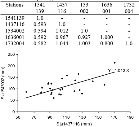
Station data correlation is set for the correlation among 5 available stations to define their slopes. The analysis is done by plotting their rainfall data and formulated linear correlation by setting the intercept is equal to zero. The two sets of rainfall data are correlated when its formulation is Y
≈
X where Y is an ordinate of 1st data set and X is an axis of 2nd data set. When Y≈
X or the slope is about unity applied, the two data sets can be treated as at-site data and the two locations are assumed to have no spatial rainfall variability and otherwise shall be treated indi-viduallly. The slopes of linear regression are summaries in Table 2 and an example of the data plotting can be seen on Fig. 3.-0.4 -0.2 0.0 0.2 0.4 0.6 0.8
10 30 50 70 90 110
Distance (KM)
C
o
e
ff
.
C
o
rr
e
la
ti
o
n
Fig. 1. Spatial correlation and distance plot for overall data among the stations
Fig. 2 shows that the data set from Sta1451139 had no co-rrelation at all to the neighboring stations since its values are about 0.50 and the data from this station will be treated indivi-dually. The rest of four stations have a good correlation by show-ing the correlation values are about one, so that at-site data will applied to the sub-region. The conclusion of the preliminary ana-lysis is that the region is divided into two sub-regions; sub-region I for northea-stern coastal area is represented by Sta1541139, and sub-region II for southwestern coastal area is represented by Sta1437116, 1636001, 1534002, and 1732004.
Table 2. The slope magnitudes for station data distribution Stations 1541
139
1437 116
153 002
1636 001
1732 004 1541139
1437116 1534002 1636001 1732004
1.0 0.593 0.594 0.592 0.582
- 1.0 1.012 0.967 1.044
- - 1.0 0.927 1.003
- - - 1.000 0.800
- - - - 1.0
Y= 1.012 X
0 50 100 150 200 250
50 70 90 110 130 150 170 190
Sta1437116 (mm)
S
ta
1
5
4
3
0
0
2
(
m
m
)
Fig. 2. Position of the stations and data correlation
Spatial data variability
The spatial rainfall variability is analyzed based annual daily maxima rainfall magnitude for 5 stations taken from the same day of record. It is assumed that the values are to be used in rainfall frequency analysis. The results of data extraction for the annual daily maxima were plotted and presented in Fig.3 and Fig.4.
Table 1. The statistical test results (u) of independence and stationary data set
Sta
2 /
α
u
Duration pattern (min)
15 30 60 120 240 480 960 1440
1437116 1534002 1541139 1636001 1732004
1.96
-0.25 -0.27 0.72 -0.16 -0.32
-0.28 -0.43 -0.11 -0.27 -0.31
-0.32 -0.40 -0.40 -0.38 -0.37
-0.33 -0.47 -0.48 -0.40 -0.35
-0.33 -0.41 -0.40 -0.35 -0.32
-0.32 -0.41 -0.35 -0.40 -0.46
-0.38 -0.36 -0.40 -0.45 -0.61
-0.43 -0.38 -0.44 -0.57 -0.78 Resource: Station data correlation.
-50 0 50 100 150 200 250 300
1980 1985 1990 1995 2000 2005
Year (1980-2004)
R
(
m
m
)
1541139 1732004 1636001 1437116
1534002 Linear (1541139) Linear (1732004) Linear (1636001) Linear (1437116) Linear (1534002)
Fig.3. Plot of data for the annual daily maxima values for Sta.1541139 and others
0 50 100 150 200 250 300 350
1980 1985 1990 1995 2000 2005
Year (1980-2004)
R
(
m
m
)
THEORY AND METHODS
Probability Weighted Moments (PWM)
Three of the more commonly can be used for parameter estimation were the method of moments (MOM), the maximum likelihood method (MLM), and the probability weighted mo-ments (PWM). Among them, the PWM method gave parameter estimates comparable to MLM estimates, yet in some cases the estimation procedure was much less complicated and the com-putation is simpler (Rao & Hamed, 2000). The PWM’s method was firstly introduced by Greenwood et al. (1979) based on the concept that the distributions whose inverse forms were expli-citly defined, such as Turkey’s lambda, may present problems in deriving their parameters by more conventional means. It has received considerable attention to the researchers and used it in their research works (Hosking et al., 1985; Hosking and Wallis, 1987; Rao & Hamed., 1997; Sveinsson et al., 2002; Kumar et al., 2005).
Hosking (1985, 1990) has defined the L-moments (Rao & Hamed, 1997). The L-moments were analogous to conventional moments and were estimated by linear combination of order sta-tistics. L-moment can also be expressed by linear combination of PWM. Thus, the procedures based on PWM and L-moments were equivalent. However, L-moments are more convenient because they were directly interpretable as measure of the scale and of the shape of probability distribution (Hosking & Wallis, 1987). Hos-king (1990) has used L-moments ratio diagram to identify under-lying parent distributions and L-moment ratios for testing hypo-theses about different probability distributions. Hosking and Wallis (1993) extended the use of L-moments and developed statistics that can be used for regional frequency analysis to mea-sure discordance, regional homogeneity, and goodness-of-fit.
Probability weighted moments Mprs was proposed by
Green-wood et al. (1979) with the following relationship.
∫
−
=
−
=
`
)
1
(
)]
(
[
}
]
1
[
)]
(
{[
0 , ,dF
F
F
F
x
F
F
F
x
E
M
s r p s r p s r p (7)where F is the cumulative distribution and there were two mo-ments to be considered:
=
=
∫
−
1 0 , 0 ,1
x
(
F
)(
1
F
)
dF
M
sα
s s (8)
=
=
∫
1 0 0 , ,1
x
(
F
)
F
dF
M
rβ
r r (9)Both
α
sandβ
rare linear in x and are of sufficient generality for parameter estimation. There are also relationship betweens
α
andβ
ras in (10) and (11).
=
∑
−
=⎟
⎠
⎞
⎜
⎝
⎛
s k k k sk
s
0)
1
(
β
α
(10)
=
∑
−
=⎟
⎠
⎞
⎜
⎝
⎛
r k k k rk
r
0)
1
(
α
β
(11)The L-moments
λ
r+1were introduced by Hosking (1985, 1990) which were linear function of PWM’s. It was more convenient than PWM’s because of the direct interpretation of the measures of scale and shape probability distribution. In terms of PWM’s,s
α
andβ
rare defined as in (12).
∑
∑
= = +=
−
=
r k k k r r k k k r r rp
p
0 * , 0 * , 1(
1
)
β
α
λ
(12) where⎟⎟⎠
⎞
⎜⎜⎝
⎛ +
⎟⎟⎠
⎞
⎜⎜⎝
⎛
−
=
−k
k
r
k
r
p
r kk
r
(
1
)
*, (13)
For given ordered sample
x
i≤
...
≤
x
n,
n
>
r
,
and n > s the unbiased sample PWM’s are calculated (Hosking 1986) using (14) and (15)
∑
=⎟⎟⎠
⎞
⎜⎜⎝
⎛ −
⎟⎟⎠
⎞
⎜⎜⎝
⎛ −
=
n i i n ss
n
x
s
i
n
a
11
/
1
(14)
∑
=⎟⎟⎠
⎞
⎜⎜⎝
⎛ −
⎟⎟⎠
⎞
⎜⎜⎝
⎛ −
=
n i i n rr
n
x
r
i
b
11
1
/
1
(15)Alternatively, consistent, but not unbiased, plotting position esti-mators are obtained by using (16) and (17)
∑
=−
=
=
n i i s n i n ss
P
x
a
1 :
1
(
1
)
ˆ
α
(16)
∑
==
=
n i i r n i n rr
P
x
b
1 : 1
β
(17) where Pi:n is the plotting position. The use of Pi:n = (i – 0.35)/nusually gives good estimates of parameters and quantiles for ge-neralized extreme value (GEV) (Hosking et al. 1985), the gene-ralized Pareto (Hosking and Wallis, 1987), and Wakeby distri-butions (Lettenmaier et al. 1987). However Hosking and Wallis (1993) recommended using plotting position estimators when using a Wakebay distribution to estimate extreme upper tail quantiles in a regional frequency analysis and to use unbiased estimators under all other circumstances. Sample L-moments (lr)
are calculated by using (12) and (13), replacing
α
sorβ
rwith their sample estima-tes as and br from (16) and (17). The L-moments ratio, which are analogous to the conventional moment ratio, are defined by Hosking (1985, 1990) in (18) and 19)
τ
=
λ
2/
λ
1 (18)
τ
r=
λ
r/
λ
2;
r
≥
3
(19)where
λ
1= measure of location;τ
= measure of scale anddis-persion (LCv);
τ
3= measure of skewness (L-Cs); andτ
4=mea-sure of kurtosis (L-Ck). Sample L-moment ratio (denoted t and tr)
are calculated by using (18) and (19), substituting sample
es-timates lr for population value
λ
r.
The L-moment ratio offer aneasy way to identify underlying, particularly skewed, distributi-ons (Hosking, 1990).
Generalized Extreme Value (GEV) Distribution
where
α
denotes a scale parameter,ε
denotes a location parame-ter, and k is the shape parameter. The PWM’s parameter esti-mates of the GEV are of the form in equation (21) (Hosking, et al., 1985).)}]
ˆ
1
(
)
1
(
1
){
ˆ
/
(
[
)
1
(
r
1u
k
r
kˆk
r
=
+
+
−
+
Γ
+
−
−
α
β
(21)The value of parameter k is given as (22) with C = (2/(3+t3 )-0.6309 (Sveinsson et al., 2002).
k
ˆ
=
7
.
8590
C
+
2
.
9954
C
2 (22)Once the value of k is obtained
α
ˆ
andµ
ˆ
are estimated by equa-tion (23) and (24) where b0, b1, b2 are the sample estimates of.
,
,
1 2 0β
β
β
α
ˆ
=
l
2k
ˆ
/{
Γ
(
1
+
k
ˆ
)(
1
−
2
−kˆ)}
(23)
u
ˆ
=
l
1+
(
α
ˆ
/
k
ˆ
){
Γ
(
1
+
k
ˆ
)
−
1
}
(24)The inverse form of the distribution function is written as (25) and by substituting F = 1 – 1/T where T is the return period, the T-year quantile estimate is obtained by using (26),
x
=
u
+
(
α
/
k
){
1
−
(
−
log
F
)
k}
(25)
x
ˆ
T=
u
ˆ
+
(
α
ˆ
/
k
ˆ
)[
1
−
{
−
log(
1
−
(
1
/
T
))}
kˆ]
(26)Generalized Logistic (GLOG) Distribution The GLOG distribution function is defined as in (27), that
F
(
x
)
=
[
1
+
{
1
−
k
((
x
−
ε
)
/
α
)}
1/k]
−1 (27)where ,
{
0
)
/
(
0
)
/
(
>
+
≤
∝<
−
<
<
≤
+
k
k
x
k
x
k
α
ε
α
α
ε
… (28)The parameter estimates and quantile are calculated using (29) to (32) with
k
ˆ
=
−
t
3 and F = 1 – (1/T) where T is the re-turn period in years.α
ˆ
=
l
2/[
Γ
(
1
+
k
ˆ
)
Γ
(
1
−
k
ˆ
)]
(29)
ε
ˆ
=
l
1+
(
l
2−
α
ˆ
)
/
k
ˆ
(30)
x
=
ε
+
(
α
/
k
)[
1
−
{
1
−
F
)
/
F
}
k]
(31)
x
ˆ
=
ε
ˆ
+
(
α
ˆ
/
k
ˆ
)[
1
−
(
T
−
1
)
−kˆ]
(32)Regional Homogeneity Current point rainfall frequency analysis techniques used in engineering design are outdated and should be developed based on regional analysis (Adamowski et. al., 1996). Regional frequ-ency analysis uses data from several sites to estimate quantiles of underlying variable at each site in the region of consideration (Cunane, 1988). The analysis involves identification of the re-gion, i.e., the site that belong to the rere-gion, testing whether the proposed region is homogeneous, choice of the distribution to fit the region data, and estimation of parameters and quantiles (Sveinsson et al., 2002). The identification of the region is something subjective and based on site characteristics; delinea-tion of the region can be approached. The site characteristics in-cludes: the latitude (o), longitude (o), alti-tude (o), concentration of precipitation (%), mean annual precipi-tation (mm), rainfall seasonability (category), and distance from the sea (m) (Smithers and Schulze, 2001). The second step is testing for regional homogeneity of the regional data that is very important for the regional frequency analysis (Dinpashoh, 2004). In practice, homogeneity is judged by the variability, among sites, of coefficient of variance Cv and /or the skew coefficient Cs, of their L-moment equivalent, or di-mensionless quantiles (Hosking, 1990; Fill and Stedinger, 1995). Fill and Stedinger (1995) studied some homogeneity tests in-cluded an index flood or Dalrymple’s test, a normalized quantile test based upon L-moment parameter estimation (X-10 test), and the method of moment Cv test (MoM-Cv test). Other L-moment based tests was H-W test proposed by Hosking and Wallis (1993) that the test would be equivalent to the X-10 test if the at-site quantiles were estimated using a fix value of shape parameter k. Based on Lu and Stedinger (1992), the X-10 test was always more powerful than the other two tests and also the X-10 test for the GEV distribution has similar power to the L-Cv regional homo-geneity test used by Hosking and Wallis (1993, 1997). The X-10 test was chosen to be used in the study since the GEV distribution was suspected to be applied to the region. Given the GEV distri-bution with L-moments parameter estimation and unit mean, so the quantiles are as in (33) that
κ
is defined using (22). The regional estimate based on at-site data and statistical test are calculated by using (34) and (35). In (33), (34), and (35),τ
ˆ
2and 3ˆ
τ
are the at-site L-Cv and L-Cs estimates,Γ
(.) is the gamma function, m is the number of sites, n is the length of data, and R denoted as regional.⎪⎩
⎪
⎨
⎧
=
+
≠
−
Γ
−
−
+
=
−0
ˆ
4139
.
2
1
0
]
)
ˆ
1
(
10536
.
0
1
[
2
1
ˆ
1
ˆ
2 ˆ ˆ 2 10κ
τ
κ
κ
τ
κ κx
(33)
∑
∑
==
m i i i i Rn
x
n
x
1 10 10ˆ
/
ˆ
(34)
=
∑
−
= − m i i R i M Lx
x
x
1 10 2 10 10ˆ
)
/
var(
ˆ
)
ˆ
(
2χ
(35)The denominator, var(
x
ˆ
10i ) can be estimated by its asymp-totic value as in (33) (Lu and Stedinger, 1992) andα
is calcula-ting using (23). The test statistics (35) has approximately a Chi-square test with (m-1) degree of freedom.var(
x
ˆ
10i)
=
(
α
2/
n
){exp[
A
]}
, where (36)
A
=
[
a
0+
a
1exp(
−
κ
)
+
a
2κ
2+
a
3κ
3]
(37) There are some methods can be used in parameter and quan-tile estimates in regional frequency analysis and one of them is a at-site method (Durrans and Kirby 2004)). This method uses all data in the homogeneous region and the data is to be treated as a single sample.RESULTS AND DISCUSSION
Identification of Homogeneous Region
State Selangor was also can be treated as one homogeneous re-gion (Masimin, 2006)
Based on above information, the area of Johore Bahru was expected to be a one homogeneous region and directed to do a sta-tistical test. There were 5 stations distributed in Johore Bahru that their samples were used to test regional homogeneity as a whole region (WR). The X-10 test using (33) to (37) was used in the study and the results are presented in Table 3 showing the values of statistical X-10 test were less than Chi-square value. It meant than the data sets for each duration pattern were passed the statistical test and the region was concluded to be a homogeneous region. The selection of the distributions will defined in the next section.
Selection of Distribution
The GEV and GLOG distributions were an appropriate selection of probability distribution based on previous study by Daud et. al. (2002) and Masimin & Harun (2006). The plotting diagram for statistical regional parameters based on L-moment for eight data sets and two types of distribution can be examined on Fig.5. Based on Fig.5, three data set for shorter duration pattern (15-, 30-, and 60-minute) follow the GLOG distribution, while the others five follow the GEV distribution as presented in Table 3.
Table 3: The results for X-10 test
Location
Duration (min)
X-10 Test 2
4 ; 9 . 0 df=
χ
Whole Region (WR)
15 30 60 120 240 480 960 1440
2.66 4.78 0.63 1.08 0.53 1.54 1.07 0.70
7.78
Parameter and Quantile Estimates
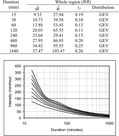
Upon the known of the probability distributions, the estima-tion of parameters and quantiles can be determined. In the study, frequency analysis was using at-site data that all data of the re-gion was to be treated as in one sample. The parameter estima-tion and quantile estimaestima-tion were only applied for GEV distribu-tion and they were determined by using (20) to (24). The values of parameter estimates for the GEV distribution were as in Table 4 and these parameters were used to calculate their quantile estimates as in Fig.6 of the plotting data.
0.10 0.14 0.18 0.22 0.26
0.10 0.15 0.20 0.25 0.30
L-Cs
L
-C
k
GEV GLOG DATA
Fig.5. Plotting diagram for L-moments parameters with GLOG and GEV distribution
Table 4: Statistical parameters based on L-moments Duration
(min)
Whole Region (WR)
L-Cv L-Cs L-Ck Distribution 15
30 60 120 240 480 960 1440
0.21 0.16 0.16 0.17 0.18 0.20 0.23 0.23
0.19 0.10 0.13 0.11 0.15 0.20 0.25 0.26
0.24 0.22 0.18 0.15 0.17 0.17 0.16 0.16
GLOG GLOG GLOG GEV GEV GEV GEV GEV
To generalize the results in constructing IDF’s family, the regretssion analysis in performing the relationship between du-ration and intensity was done and the power relationship was the appropriate one as in (38) where a and b were parameters to be defined.
I
T=
at
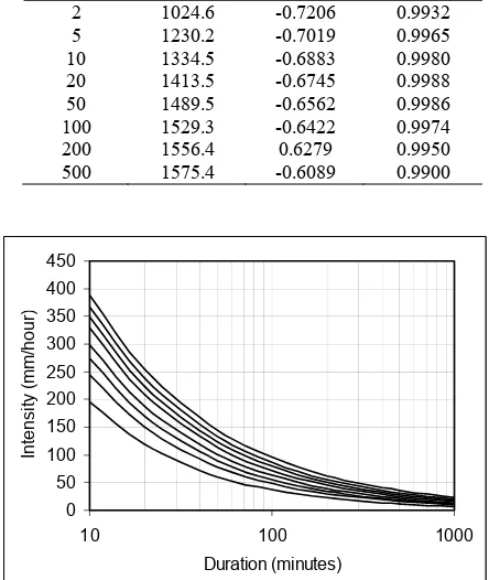
b (38) In (38), IT = rainfall intensity for the T-year return period(mm/hour); t = duration equal to the time concentration (minu-tes); a and b = parameters. The results of regression analysis were presented in Table 5 showing the values of a, b, and R2 for every proposed return period. Looking at the value of R2 that mostly about 0.99, it meant that the power relationship for IDF’s family was very rational. The final result of IDF’s family was presented in Fig.7.
Table 4. Parameter estimates based on the GEV distribution Duration
(min)
Whole region (WR)
α
ˆ
u
ˆ
t3 Distribution15 30 60 120 240 480 960 1440
9.33 10.73 13.88 20.03 23.68 27.95 34.42 37.47
27.94 39.58 53.45 65.55 29.41 86.05 95.55 105.47
0.19 0.10 0.13 0.11 0.15 0.20 0.25 0.26
GEV GEV GEV GEV GEV GEV GEV GEV
0 50 100 150 200 250 300 350 400
10 100 1000
Duration (minutes)
In
te
n
s
it
y
(m
m
/h
o
u
r)
Fig.6. Plotting data for the intensity quantile estimates
Fig.7 was the IDF’s curves family that developed based on 5-minute incremental rainfall data; it was needed to compare the cur-ve with those of Mononobe method as in (1). By applying the daily (1440-minute) rainfall data for the return period T = 100
Mononobe method gave an over estimate value about 10% for the common duration pattern applying in urban drainage projects that was 30 to 100 minutes. It is noted that the rational method is only applied to the area less than 600 acres or 248 ha and for the area greater than those, it is recommended to use hydrograph analysis with the input is a fractional rainfall data. It is a future research topic of the writer.
Table 5: Parameter estimates for power relationship
T
(year) a b R2
2 5 10 20 50 100 200 500
1024.6 1230.2 1334.5 1413.5 1489.5 1529.3 1556.4 1575.4
-0.7206 -0.7019 -0.6883 -0.6745 -0.6562 -0.6422 0.6279 -0.6089
0.9932 0.9965 0.9980 0.9988 0.9986 0.9974 0.9950 0.9900
0 50 100 150 200 250 300 350 400 450
10 100 1000 Duration (minutes)
In
te
n
si
ty
(m
m
/h
o
u
r)
Fig.7. The family of intensity duration frequency (IDF-curves)
0 100 200 300 400 500
10 100 1000
Duration (minutes)
In
te
n
s
it
y
(
m
m
/h
o
u
r)
Cal. Mon.
Fig.8. The comparison for IDF-curve based on calculation and Mononobe method.
CONCLUSIONS
As the conclusion, the study revealed some of the following information
1.The whole region of the area of Johore Bahru can be treated as one regional homogeneous area that matching to the study by Daud et. al. (2002).
2.Two types of probability distributions, GEV and GLOG distributions, were applied to the all duration pattern rainfall data in Johore Bahru.
3.Looking at the statistical L-moments analysis, the higher L -Ck, the sample tends to follow the GLOG distribution and it follows the GEV distribution for the lower L-Ck.
4.The terms of quantile estimates that it was intended to use in design storms development, GEV distribution was proposed to be used in analysis.
5.By comparing the IDF-curve proposed by Mononobe method that predicting the intensity based daily rainfall data, both IDF curves were identical with Mononobe method gave the result of 10% over estimate.
The general conclusion of the study of design storms deve-lopment is that the homogeneous region and the type of proba-bility distribution are identified including their quantile estima-tes. Since the study is using the rational method with its limi-tation, it is identified that the further study related to the topic of design storms is a fractional rainfall characteristics as an input for hydrograph analysis that to be applied for greater coverage areas.
Acknowledgement
The writers want to deliver thousand thanks going to UNSYIAH-Banda Aceh, Indonesia, UTM-Johore Bahru, Malay-sia, especially for TPSDP-PROJECT for the funding that this study become a reality. Special appreciation is going to JPS Am-pang, Kuala Lumpur, Malaysia for the availability 5-minute incremental rainfall data that the knowledge of theory becomes visible practice.
REFERENCES
Adamowski, K., Alila, J. & Pilon, P.J. (1996). ”Regional rainfall distribution for Canada.” Atmospheric Research 42, 75-88. Adamowski, K. and Bougadis, J. (2003). “Detection of trends in
annual extreme rainfall.” Hydrol. Processs. 17, 3547-3560. Berndtsson, R. & Niemczynowics, J. (1986). “Spatial and
tem-poral characteristics of high-intensive rainfall in northern Tunisia.” Journal of Hydrology, 87, 285-298.
Burn, D.H. (1990). “Evaluation of regional flood frequency ana-lysis with a region of influence approach.” Water Resources Research, 26(10), 2257-2265.
Chow, V.T. (1964). Handbook of applied hydrology, McGraw-Hill Book Co., New York.
Cunnane, C. (1988). “Methods and merits of regional flood fre-quency analysis.” J. Hydrology, 100, 269-290.
Dinpashoh, Y., Fakheri-Fard, A., Moghaddam, M., Jahanbakhsh, S. & Mirnia, M. (2004). “Selection of variables for the pur-pose of regionalization climate using multivariate methods.”
J. Hydrology, 297, 109-123.
Daud, Z.M., Mohd Kassim, A.M., Mohd Desa, M.N., & Nguyen, V.T.V. (2002). “Statistical analysis of at-site extreme rainfall process in Peninsular Malaysia.” Proc. of 4th Int. Conference of FRIEND, Cape Town, March 2002, IAHS Publication (274), 1-8.
Durrans, S.R. & Kirby, J.T. (2004). “Regionalization of extreme precipitation estimates for the Alabama rainfall atlas.” Jour-nal of Hydrology, 295,101-107.
Fill, H.D. & Stedinger, J.R. (1995). “Homogeneity tests based upon Gumbel distribution and a critical appraisal of Dalrym-ple’s test.” J. Hydrology, 166, 81-105.
Greenwood, J.A., Landwehr, J.M., Matalas, N.C., & Wallis, J.R. (1979). “Probability weighted moments: Definition and rela-tion to parameters of several distriburela-tions expressable in in-verse form.” Water Resources Research, 15(5), 1049-1054. Hosking, J.R.M., Wallis, J.R. & Wood, E.F. (1985). “Estimation
Hosking, J.R.M. & Wallis, J.R. (1987). “An ‘index flood’ proce-dure for regional rainfall frequency analysis.” Eos Trans. Am. Geophys. Un., 68, 312.
Hosking, J.R.M. & Wallis, J.R. (1987). “Parameter and quantile estimation for the generalized Pareto distribution.” Techno-metrics, August 1987, 29 (3), 339-349.
Hosking, J.R.M, (1990). “L-moments: Analysis and estimation of distributions using liner combinations of order statistics.” J. R. Stat. Society, 52 (1), 105-124.
Hosking, J.R.M. & Wallis, J.R. (1993). “Some statistics useful in regional frequency analysis.” Water Resources Research, 29(2), 271-281.
Hosking, J.R.M. (1996). Fortran routines for use with the method of L-moments. RESEARCH REPORT, IBM Research Divisi-on, Yorktown Heights, NY 10598.
Kottegoga, N.T. & Rosso, R. (1997) Statistics, probability, and reliability for civil and environmental engineers, The Mc Graw-Hill Companies, Inc., New York, USA.
Kumar, R. & Chatterjee, C. (2005). “Regional flood frequency analysis using L-moments for North Brahmaputra region of India.” J. Hydrol. Engg., 10(1), 1- 7.
Lettenmaier, D.P., Matalas, N.C. &Wallis, J.R. (1987). “Estima-tion of parameters and quantiles of Wakeby distribu“Estima-tion, part 1 and 2.” Water Resources Research, 15(6), 1361-1379. Lu, L.H. & Stedinger, J.R. (1992). “Sampling variance of
norma-lized GEV/PWM quantile estimators and a regional homo-geneity test.” J. Hydrology, 138, 223-245.
Lu, L.H. & Stedinger, J.R (1992). “Variance of two and three-parameter GEV/PWM quantile estimators: formulae,
con-fidence intervals, and a comparison.” J. Hydrology, 138, 247-267.
Masimin & Harun, S. (2006). “Analysis for annual maximum pre-cipitation series for State of Selangor using probability weigh-ted moments.” Proc. of Hydrological Sciences for Managing Water Resources in the Asian Developing World Con-ference, Guangzhou, P.R. China.
Mohd. Kasim, A.H., & Way, L.K. (1995). Frequency analysis of annual maximum rainfall for the Klang river basin using GEV distribution. Faculty of Civil Engineering, Universiti Teknolo-gi Malaysia, Johor Bahru, Malaysia.
Rao, A.R & Hamed, K.H. (1997). ”Regional frequency analysis of Wabash river flood data by L-Moments.” J. Hydrol. Engg.,
2(4), 160-179.
Rao, A.R & Hamed, K.H. (2000). Flood frequency analysis. CRC Press, New York, USA.
Rao, A.R. & Srinivas, V.V. (2006). “Regionalization of water-sheds by fuzzy cluster analysis.” J. Hydrology, 318, 57-79. Smithers, J.C. & Schulze, R.E. (2001). “A methodology for the
estimation of short duration design storms in South Africa using regional approach based on L-moment.” J Hydrology, 241, 42-52.
Sosrodarsono, S. & Takeda T. (1980). Hidrologi untuk Pengair-an, Pradnya Paramita, Jakarta.
Sveinsson, O.G.B., Salas, J.D. & Boes, D.C. (2002). “Regional frequency analysis of extreme precipitation in Northeastern Colorado and Fort Collins flood of 1997.” J. Hydrol Engg., 7(1), 49-63.