T
TTIIINNJNJJAAAUUUAANANN PPPUUSUSSTTTAAAKKAKAA
DEVELOPING DECISION SUPPORT SYSTEM FOR WATER
RESOURCES MANAGEMENT UNDER UNCERTAINTY
Wirsal Hasan dan Herman Mawengkang
Doctoral Program of Management of Natural Resources and Environment, The University of Sumatera Utara.
(Presented at 2nd Regional Converence on Ecological and Environmental Modelling on August 28-30, 2007 in Penang, Malaysia)
ABSTRACT
Water Resource (WR) management problems with a multiperiod feature are associated to mathematical optimization models that handle thousandss of constraints and variables depending on the level of adherence required to reach a significant representation of the system. Moreover these problems are typically characterized by a level of uncertainty about the value of hydrological exogenous inflows and demand patterns. In this paper we present a scenario analysis approach to perform water system planning and management under climatic and hydrological uncertainty. A decision support system (DSS) with a graphical interface allows the user a friendly data-input phase and result analysis. Different generation techniques can be used to set up and analyze a number of scenarios. Uncertainty is modeled by a scenario-tree in a multistage environment, which includes different possible configurations of inflows in a wide time-horizon. The aim is to indetify trends and essential features on which to base a robust decision policy.
Keywords: Water resources management, Decision support system
INTRODUCTION
Water Resource (WR) management problems with a multiperiod feature are associated to mathematical optimization models that handle thousandss of constraints and variables depending on the level of adherence required to reach a significant representation of the system. Moreover these problems are typically characterized by a level of uncertainty about the value of hydrological exogenous inflows and demand patterns. On the other hand inadequate values assigned to them could invalidate the results of the study. When the statistical information on data estimation is not enough to support a stochastic model or when probabilistic rules are not available, an alternative approach could be in practice that of setting up the scenario analysis technique. Dembo [1991], Rockafellar [1991], and Mawengkang [2007]. In WR analysis a scenario can represent a possible
"robust-barycentric" solution can be then obtained by a postprocessor phase applied to sub-problems solutions.
A WR model is usually defined in a dynamic planning horizon in which management decisions have to be made either sequentially, by adopting a predefined scenario independently.
Extending the analysis to a set of scenarios, an aggregation condition will guarantee that the solution referred to a period t is independent of the information that is not yet available. In other words, model evolution is only based on the information available at the moment, a time when the future configuration may diversify. The availability, in the proposed DSS, of an efficient computer graphical interfaces, designed to facilitate the use of models and database, help end-users to evaluate the best choice in a friendly-to-use way starting from physical system to reach a robust solution for environmental water resources management problem. The proposed tool can perform scenario analysis by generating a scenario-tree structure.
WATER RESOURCES DYNAMIC MODEL
In this section we formulate a water resources management model in a deterministic framework, i.e. having a previous knowledge of the time sequence of inflows and demand. We extend the analysis to a sufficiently wide time horizon and assuming a time step (period),
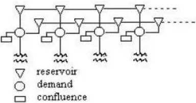
t. The scale and number of time-steps considered must be adequate to reach a significant representation of the variability of hydrological inflows and water demands in the system. Referring to a "static" or single-period situation, we can represent the physical system by a direct network (basic graph), derived from the physical sketch. Nodes could represent sources, demands, reservoirs, groundwater, diversion canal site, hydropower station site, etc. shows a physical sketch and the basic graph of a simple water system. A dynamic multiperiod network derived by replicating the basic graph for each period supports the dynamic problem. We then connect the corresponding reservoir nodes for different consecutive periods by
additional arcs carrying water stored at the end of each period. Figure 1 shows a segment of a dynamic network generated by a simple basic graph.
Figure 1. Segment of a Dynamic Network
Even if the aim of this paper is not to detail the components of the mathematical model, we give a formulation of a reduced model that can be adopted to formalize the uncertainty in water resources management. To illustrate our approach, we adopt a deterministic Linear Programming (LP) described in the next section.
Definition of Water Resources Optimization Model Components
Even if it is quite impossible to define a general mathematical model for water resources planning and management problem, our DSS allows to take into account the components of a system as general as possible based on the most typical characterization of this type of models. Different components can be considered or ignored updating constraints and objective. In this paper we describe only some of them due to limited space allowed. More detailed description of this approach can be found in Sechi and Zuddas [2000], Onnis et al. [1999]. In the following we refer to the dynamic network G = (N, A) where N is the set of nodes and A is the set of arcs. T
represents the set of time-steps t.
Identification of Hydraulic Network Components and Sets
Nodes (subsets ofN):
res set of reservoir nodes: these
represent surface water resources with
storage capacity.
consumptive or non-consumptive water demand nodes
hyp set of hydroelectric nodes: they are
non-consumptive nodes associated with hydroelectric plants
con set of confluence nodes: such as
river confluence, withdraw connections for demands satisfaction, etc.
Other sets of nodes can represent groundwater, desalinization, wastewater-treatment plant,among others.
Arcs: (subsets ofA)
R set of weighted arcs: these represent arcs whose flow produce a cost or a benefit per unit of flow, such as conveyance work arcs, artificial channels among others;
TRF set of transfer arcs: these represent transfer works in operational or in project state;
Other sets of arcs are present in the tool referred to emergency transfers, spilling arcs, among others
Required Data
Data marked with (+) refer to operational state (existing works with a
known dimension) while data marked with (*) are refer project state
(works to be constructed). Unmarked data refer to operational and project state.Required data for a reservoir j:
Yjmax (+) max storage volume for inter-periods transfer.
ρt
jmax (+) ratio between max volume usable in each period t and the reservoir capacity.
ρt
jmin (+) ratio between min stored
volume in each period and reservoir capacity.
δj gradient of the relationship between the reservoir surfaces and volumes. in the same way can be defined required data for industrial and irrigation demands; required data for a hydroelectric power station j:
data for a confluence node j: Itj hydrologic input (if arcs are
natural streams); required data for a transfer arc a:
Fa (+) transfer capacity ρt
amax (+) ratio between max transferred
volumes and capacity
ρtamin (+) ratio between min transferred
volumes and capacity
ca operating cost.
Famax (*) max transfer capacity
Famin (*) min transfer capacity γa (*) construction cost
Decision Variables and Constraints
ytj_ portion of stored water at reservoir k at the end of period t that can be used in next periods. The corresponding constraints, for each time period t is:
ρt
kminYjmax < ytj_<_ρtjmax_Yjmax_
this constraints ensures that, in each period, the used volume of the reservoir k be in the prescribed range. In a operational state is a data while in a project state it is a decision variable. In the last case it is bounded by:
mj < Yjmax < Mj, ∀ j∈ res ptj_ water demand at civil demand center j
in period t. The corresponding constraints, for each time period t is
ptj = πtj dtj Pj, ∀j∈ dem
this constraints ensures the fulfillment of the demand in each period, no matter if coming from the system or from a dummy resources. In a operational state Pj is a data while in a project state it is a decision variable. In the last case it is bounded by:
Pjmin < Pj < Pjmax___ , ∀ j∈
dem
Variable and constraints are defined in the same way for other demand sets.
htj water trough hydropower plant j (hydroelectric power station) in period t. The corresponding constraints, for each time period t is:
htj < πtjαj Hj,∀j∈ hyp
this constraints expresses the dependence of flow on production capacity. In a operational state Hj is a data while in a project state it is a decision variable. In the last case it is bounded by:
Hjmin< Hj< Hjmax__, ∀ j∈hyp
xtj flow on arc a. In case of a transfer arc
a, the corresponding constraints, for each time period t is:
ρt
aminFa < xta_<_ρtamax Fa, ∀a ∈ TRF
this constraints ensures that, in each
period, the transferred volume in arc a
be in the prescribed range. In a operational state _Fa is a data while in a project state it is a decision variable. In the last case it is bounded by:
Famin < Fa <_Famax, ∀a ∈ TRF
Variable and constraints are defined in the same way for other arc sets. Referring to the multiperiod dynamic network structure, mass balance constraints are defined in each node i∈N. Moreover, lower and upper bounds constraints are defined in some arcs a∈A to represent some particular limits as for transfer arcs
TRF.
Objective Function
The objective function considers weights on variables, that is costs and benefits as well as penalties, associated to flow and project variables. Following simplified notation defined in this paper the objective function is the following:
Σj ∈ res γj Yjmax- Σj ∈ dem βj Pj + Σj∈ dem γj Hj+ Σa
∈ TRF γa Fa + Σa ∈ Rca xta
Compact Deterministic LP Model
As is well known in LP theory, the described mathematical model can be expressed in a compact standard form as follows:
min c x s.t. A x = b l < x <_u
where:
x represents the vector comprehensive of all operating and projects variables;
c represents the vector comprehensive of all weights on operating and projects variables;
l and_ u represent vectors comprehensive of all lower and upper bounds on operating and projects variables;
b represent the vector of R.H.S.;
A x = b represent the set of all constraints. In what follows for the sake of simplicity we adopt the compact model to illustrate the scenario approach.
DYNAMIC MODEL
The presented model is named chance-model to put in evidence that it is not stochastic based but, due to the impossibility to adopt probabilistic rules, try to represent a set of possible performances of the system as uncertain parameters vary. When a set of different and independent scenarios are generated, the structure of the chance-model is based on scenario aggregation
condition generating a graph structure named "scenario tree".
Further Components in Chance Model and Scenario-tree Generation
Data defined for deterministic model are required for each scenario in the chance model plus the further data:
G set of synthetic hydrological sequences (parallel scenarios) wg weight assigned to a scenario g ∈ G
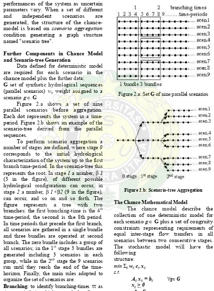
Figure 2.a shows a set of nine parallel scenarios before aggregation. Each dot represents the system in a time-period. Figure 2.b shows an example of the scenario-tree derived from the parallel sequences.
To perform scenario aggregation a number of stages are defined, where stage 0
corresponds to the initial hydrological characterization of the system up to the first branch time-period. In the scenario-tree this represents the root. In stage 1 a number, β 1
(3 in the figure), of different possible hydrological configurations can occur, in stage 2 a number, β 1 ∗β2 (9 in the figure), can occur, and so on and so forth. The figure represents a tree with two branches: the first branching-time is the 4th time-period, the second is the 8th period. In time periods that precede the first branch, all scenarios are gathered in a single bundle and three bundles are operated at second branch. The zero bundle includes a group of all scenarios; in the 1st stage 3 bundles are generated including 3 scenarios in each group, while in the 2nd stage the 9 scenarios run until they reach the end of the time-horizon. Finally, the main rules adopted to organize the set of scenarios are:
Branching: to identify branching-times ττ as time- periods in which to apply bundles on parallel sequences, while identifying the
stages in which to divide the scenario horizon.
Bundling: to identify the number, ββ τ , of bundles at each branching-time.
Grouping: to identify groups, to include in each bundle.
Figure 2.a: Set G of nine parallel scenarios
Figure 2.b: Scenario-tree Aggregation
The Chance Mathematical Model
The chance model describe the collection of one deterministic model for each scenario g ∈ G plus a set of congruity constraints representing requirements of equal inter-stage flow transfers in all scenarios between two consecutive stages. The stochastic model will have the following
structure:
min Σg wg cg xg
s.t.
Ag xg = bg ∀g∈ G
xg > 0
x* ∈ S
constraints on inter-stage flows. An alternative formulation of the objective function can be expressed as
min Σg wg||cg ( xg - xg* )||
where xg* is an optimal policy expected by
water manager.
This kind of model can be solved by decomposition methods such as Benders decomposition techniques, which exploit the special structure of constraints. Cai et al. [2001]. When the size of the problem becomes huge, it is possible to resort to parallel computing. The resolution approach can be described as a three-phase algorithm:
− scenario-tree generation and identification of the chance model;
− resolution of the chance model. At the end of this phase we obtain a solution-set xG = Ugxg;
− obtaining a "robust" solution by a postprocessor on the solution-set.
The postprocessor refers to identify the most performable solution or the most profitable solution or the most "barycentric" solution, and so on, depending on the features of the system and on the end-user point of view.
DECISION SUPPORT SYSTEM (DSS)
DSS can be defined as an interacting computer-based system that helps the decision maker in the use of data and models in the solution of unstructured problems in the environmental domain DSS features • assist managers in
unstructured/semi-structured tasks
• support rather than replace the human DM • improve the effectiveness rather than the
efficiency
• combine the use of models or analytical techniques with data access functions • Emphasise flexibility and adaptability to
respect changes in the decision context • Focus on features to enhance user
interaction
The Decision Support System has been developed in order to
- be friendly to use in input phase, in scenarios setting and in processing output results;
- be easy to modify system
configuration and related data to perform sensitivity analysis and to process data uncertainty;
- prevent obsolescence of the optimizer exploiting the standard input format in optimization codes.
A graphical interface allows performing scenario analysis starting from physical system following the main steps:
- time period definition and scenario settlement;
- system elements characterization; - connections topology and transfer
constraints.
- links to hydrological data and demand requirements files;
- planning and management rules definition;
- benefits and costs attribution; - call to optimizers;
- output processing.
CONCLUSION AND PERSPECTIVES
This paper is aimed to give a contribution to the mathematical optimization of water resources systems, when the role of uncertainty is particularly important. In such a problem, which involves social, economical, political, and physical events, no probabilistic description of the unknown elements is available, either because a substantial statistical base is lacking or because it is impossible to derive a probabilistic law from conceptual considerations. Another not secondary aim planning the presented approach for WR analysis is to create a tool to help water managers in a DSS context, friendly to use but able to take into account the improvements made in the field of computer science and operation research. The state of the art in Mathematical Programming codes evolves continuously producing algorithms that improve computational efficiency thanks to new methodologies and computer science development. See MINOS(1982). The standard input format allows to insert the best state-of-the-art codes in the DSS.
Cai, X., D.C. McKinney, L.S. Lasdon, D.W. Watkins Jr., Solving Large Nonconvex Water Resources Management Models using Generalized Benders Decomposition, Operations Research, 2, 235-245, 2001.
Dembo, R. Scenario Optimization, Annals of Operations Research, 30, 63-80, 1991. Loucks, D. P., J. R. Stedinger, and D. A. Haith.. Water Resource Systems Planning and Analysis. Prentice Hall, Englewood Cliffs, NJ, 1981.
Murtagh,B.A. and M.A. Saunders, A Projected Lagrangian Algorithm and Its Implementation for Sparse Nonlinear Constraints. Mathematical Programming Study 16, 84-117
Mawengkang, H and Suherman, A heuristic Method of Scenario Generation in Multi-stage Decision Problem Under Uncertainty, J.Sistem Teknik Industri, vol. 8, 2007
Onnis, L., G.M Sechi,. and P Zuddas, Optimization Processes under Uncertainty, A.I.C.E, Milano, 283-244, 1999.
Rockafellar, R.T. and R.J.-B.Wets. Scenarios and Policy Aggregation in Optimization Under Uncertainty,
Mathematics of operations research, 16, 119-147, 1991.
Sechi G.M. and Zuddas, P., WARGY: Water Resources System Optimization Aided by Graphical Interface, in (.R. Blain, C.A. Brebbia, eds.), Hydraulic Engineering Software, WIT-PRESS, 109-120, 2000.