Aerodynamic stability of road vehicles in dynamic motion.

(1)

The Seventh International Colloquium on Bluff Body Aerodynamics and Applications (BBAA7) Shanghai, China; September 2-6, 2012

Aerodynamic stability of road vehicles in dynamic motion

S.Y. Cheng

a

, M. Tsubokura

a

, T. Nakashima

b

, Y. Okada

a,c

, T. Nouzawa

c a

Graduate School of Engineering, Hokkaido University, Japan b

Graduate School of Engineering, Hiroshima University, Japan c

Vehicle Testing & Research Department, Mazda Motor Corporation, Japan

ABSTRACT: A method for dynamic coupling simulation of flow and vehicle motion was devel-oped based on large eddy simulation technique with moving boundary methods. The method was applied to investigated the aerodynamic stability of vehicle under a transient driving situation. A coefficient to quantify the aerodynamic damping was defined. For the sedan-type, simple body models investigated, the underbody provides the highest proportion of aerodynamic damping. However, it is the trunk deck contribution that causes the different damping magnitudes in the models with distinct A- and C-pillar geometrical configurations.

KEYWORDS: Aerodynamics, transient, LES, vehicle, stability, damping, pitching.

1 INTRODUCTION

In principle, automotive aerodynamics comprises the drag, lift, and side force coefficients, in conjunction with the rolling, yawing, and pitching moment coefficients. In real-world situation, the aerodynamic forces and moments which act on a vehicle are of transient nature. However, development of vehicle aerodynamics to date has mainly been focused on the steady-state com-ponents, particularly the drag coefficient, Cd. This coefficient can only be used to evaluate

per-formances related to fuel efficiency and top speed, and provides no indication in regard to the

vehicle’s performance in terms of stability.

To consider the stability factors under the effect of transient aerodynamics, several assessment methods have been proposed in the literature. These methods rely on either drive test (e.g. How-ell and Le Good, 1999; Okada et al, 2009) or wind tunnel measurement (e.g. Aschwanden et al, 2006). The former can only be performed after a development mule is produced, while the latter requires a complex test rig to manipulate the vehicle motion for a dynamic assessment. In addi-tion, due to limited numbers of probe that can be attached to the test vehicle without altering the surrounding flow, drive test and wind tunnel measurement provide very limited flow information about the test. The lack of flow information could impede detailed flow analysis which is needed for identifying the underlying mechanism.

To overcome these limitations, thus the main objective of the present study is to develop a nu-merical method for the assessment of vehicle aerodynamic stability performance under a transi-ent driving situation. The method allows manipulation of vehicle body motion during flow simu-lation, and quantification of vehicle stability performance on the basis of the aerodynamic damping generated by the vehicle, which is depending on the vehicle's body shape configuration.

2 SIMPLE BODY MODELS

(2)

In general, both models are the 1:20-scale, simple bluff-bodies with same height h, width w, and length l measurements of 65, 80, and 210 mm, respectively. The models have A- and C-pillars with the same slant angles of 30° and 25°, respectively, which are based on the configurations of real vehicle.

Figure 1. Simple body models: (a) model A (Top) and model B (Bottom); (b) Designations of body part.

3 NUMERICAL METHODS

3.1 Governing equations

The LES solves the following spatially filtered continuity and Navier-Stokes equations:

0

and strain rate tensor. The over-bar denotes a spatially filtered quantity. Meanwhile, the standard Smagorinsky model is adopted to model the subgrid-scale (SGS) eddy viscosity vSGS of Eq. (2).

(3)

the centerline of ASMO model and the flow field around a full-scale production car (including a complicated engine room and under-body geometry).

3.2 Discretization

The governing equations were discretized by using the vertex-centered unstructured finite-volume method. We adopted the second-order central differencing scheme for spatial deriva-tives, and exploited the blending of 5% first-order upwind scheme for the convection term for numerical stability reason. Meanwhile, pressure-velocity coupling was preserved by the SMAC (simplified marker and cell) algorithm.

For time advancement, the LES adopts the Euler implicit method. This is because an implicit scheme can accommodate larger time difference than an explicit one without causing numerical instability, especially in the case of a vehicle simulation in which the velocity and mesh size vary strongly. With larger permissible time difference (∆t = 1×10-5 s), the scheme needs lesser time steps (hence, shorter simulation time) to obtain a reliable time- and phase-averaging statistic. Such feature is important in dynamic LES cases, because they normally need over hundred thou-sand of time steps to obtain an adequate phase-averaging statistic. In the present study, the com-putations took about 50,000 simulation steps (over five pitching cycle) to reach a stable periodic condition and the subsequent 150,000 steps to covers 15 cycles of pitching oscillation for obtain-ing an adequate phase-averagobtain-ing statistic.

3.3 Computational domain and boundary conditions

The computational domain resembles a rectangular wind-tunnel test section. Its cross section co-vers 1.52l on both sides of the model and height of 2.23l. This set-up produces a small blockage ratio of 1.53%, which is well within the typically accepted range of 5% in automotive aerody-namic testing (Hucho and Sovran, 1993). The model was situated near the domain floor at a ground clearance of 0.071l. The inlet boundary was located 3.14l upstream, while the outlet boundary was 6.86l downstream.

At the inlet boundary, the air flow approaches at a constant velocity of 16.9 m/s, corresponding to Re of 2.3 × 105 (based on vehicle length l). Meanwhile, a zero-gradient condition is imposed at the outlet boundary. The ceiling and side boundaries of the domain were treated with free-slip wall-boundary condition. The ground surface is divided into two zones. The upstream zone (which covers 3l from the inlet boundary) is defined as a free-slip wall condition to avoid bound-ary-layer formation. This setting simulates the wind-tunnel experimental condition, thus ensure the consistency of flow condition between the LES and wind tunnel test so that direct compari-son between their results is allowed during validation. The remaining ground and vehicle surface are treated with the logarithmic-law (y+ > 11.63) or linear law functions (y+ < 11.63) depending on the obtained y+ values. We have found that the very fine spatial resolution adopted produces the y+ < 4 around the vehicle surface, thus the estimation is by the linear law function, which cor-responds to the no-slip wall condition.

4 FORMULATION OF AERODYNAMIC DAMPING COEFFICIENT

4.1 Periodic-pitching-oscillation condition

(4)

 

0 1sin t

     _,

 

t 2 f t_p (4)

By setting θ0 and θ1 equal to 2°, the vehicle models were forced to oscillate at amplitude of 2°.

Although this value is larger than the range a vehicle would encounter under normal driving conditions, it has the advantage of producing more distinct aerodynamic damping effect in vehi-cles of different stability characteristics. Thus make it easier to interpret the underlying physical mechanism. Frequency fp was 10 Hz, which corresponds to a Strouhal number (St) of 0.13,

nor-malized by l and Uinlet. This value was chosen in consideration of the St of 0.15 obtained by road

test by Okada et al. (2009). Figure 2 shows the sign convention for aerodynamic pitching mo-ment M and angle θ.

Figure 2. Sign convention for M and θ.

4.2 Periodic-pitching-oscillation condition

The estimated phase-averaged pitching moment <M>p can be decomposed into steady and

un-steady components. The equation for phase-averaged pitching moment <M>p in terms of pitch

angle θ is given as the following expansion:

0 1 2 3

p

M C C C C

      (5)

where, respectively, the single dot and double dots in the third and fourth terms indicate the first and second derivatives with respect to time t. Both C0 and C1 are static components; the former

denotes the pitching moment M at zero pitch, while the latter describes the quasi-static behavior by taking into account the pitch-angle variation in a static manner. C2 is associated with

aerody-namic damping, and C3 is an added moment of inertia that is proportional to angular

accelera-tion.

Substituting Eq. (4) into (5) and rearranging gives:





 

3

 

2

0 1 0 1 2 1sin 2 1 2cos

p p p

M C C C  f C   t  f C  t

    __  __  (6)

The above equation can then be rewritten by using new parameters, namely, Mstat, Mdis and Mang

as

 

stat sinsin coscos

M p M M  t M  t

     (7)

where, Mstat is a constant, which set the baseline for the <M>p. Mdis is the amplitude of the term

which in-phase with the imposed pitching displacement, and Mang is the amplitude of the term

(5)

4.3 Definition of aerodynamic damping coefficient

During one pitching cycle, time t varies from 0 to 2π/ω. Hence, the work done by the aerody-namic pitching moment M on the vehicle model during one pitching cycle is:

 

Substituting Eq. (7) and (10) into eq. (11), the work done during one pitching cycle becomes

 

The result of the integration reveals that the net work done on the vehicle by aerodynamic pitch-ing moment M over a pitching cycle is depends on the component in-phase with the angular ve-locity Mang. In Eq. (10), θ1 and π are given. Hence, the parameter Mang reflects the dynamic

re-sponse of the vehicle. This parameter can be presented in a non-dimensional form. If normalized in a similar manner to the pitching-moment coefficient, it becomes:

ang

damp the pitching oscillation, whereas a positive value enhances the vehicle motion (i.e. negative damping). The coefficient thus enables quantitative evaluation of vehicle stability; therefore, it is

termed “aerodynamic-damping coefficient.”

5 RESULTS AND DISCUSSIONS

5.1 Aerodynamic damping coefficient of simple body models

Figure 3 shows the <M>p as a function of phase angle φ for models A and B. The coefficients in

Eq. (7) are obtained by fitting the equation to the <M>p data set by nonlinear least squares

re-gression. Solid lines in Figure 3 are the fitted functions for the two models. Table 1 summarizes the corresponding CAD for comparison. As shown in the table, the aerodynamic damping

coeffi-cient CAD for the two models are negative, implying a tendency to resist the pitching motion.

Be-tween them, however, model B has a higher aerodynamic-damping coefficient CAD, by about

(6)

Figure 3. Phase-averaged M and fitted functions.

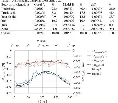
Table 1. Aerodynamic damping coefficient CAD

Body part resignations Model A % Model B % diff % Underbody -0.0309 78.6 -0.0347 60.6 -0.00376 21.0 Trunk deck -0.00205 5.2 -0.0100 17.5 -0.00795 44.4 Rear-shield -0.000350 0.9 -0.00709 12.4 -0.00674 37.7 Roof -0.00658 16.7 -0.00607 10.6 0.000513 -2.9 Base 0.000162 -0.4 0.000128 -0.2 -0.0000342 0.2 Panel 0.000376 -1.0 0.000453 -0.8 0.0000769 -0.4 Overall -0.0394 100.0 -0.0573 100.0 -0.0179 100.0

Figure 4. Phase-averaged M and fitted functions.

(7)

particularly the trunk deck. Figure 4 shows that the curves of trunk deck fitted function of the two models have very similar phase shift. However, the relatively low trunk deck contribution in model A is caused by the smaller fluctuation amplitude.

5.2 Aerodynamic damping mechanism

5.2.1 Main aerodynamic damping contribution

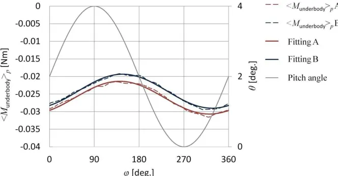
The underbody has the highest damping contribution due to two reasons: First, the dynamic ef-fect, i.e. vehicle motion, has caused the phase of phase-averaged underbody pitching moment <Munderbody>p curve to shift (by about 128° and 134° in model A and model B, respectively) at the

pitching oscillation frequency (see Figure 5), thus produces a negative Mang; Second, its

relative-ly large surface area and moment arm produce a significantrelative-ly larger Mang magnitude then other

body parts.

Figure 5. <Munderbody>p and fitted functions of underbody: (a) Model A; (b) Model B.

The behavior of <Munderbody>p curve can be explained by first considering the quasi-steady flow

(8)

Figure 6. Phase-averaged velocity distribution at underfloor clearance and static pressure of underbody; model B.

5.2.2 Comparison between two aerodynamic configurations

Figure 4 shows that the phase-averaged trunk deck pressure lift <Lprs_deck>p and phase-averaged

trunk deck pitching moement <Mdeck>p curves of the two models are matching well, implies that

the <Mdeck>p is mainly caused by the trunk deck surface static pressure. Ideally, the pressure

force should be in-phased with the angular velocity of pitching to produce a maximum damping. That is, the <Lprs_deck>p peaks at φ = 180°, and reaches the minimum at φ = 0 or 360°. The

<Lprs_deck>p curves for the two models nearly meet this criterion, with only a slight phase shift.

Hence, the CAD obtained from the two models are having the same sign. However, the relatively

large fluctuation range in model B has resulted in a higher damping magnitude.

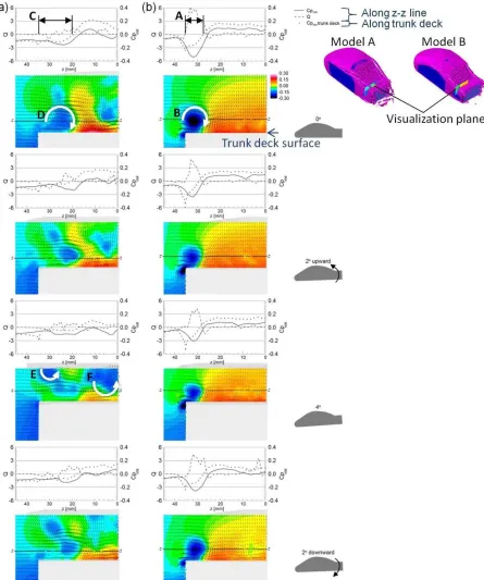
Next, we discuss the reasons that cause the trends observed in Figure 4. As shown, model B has a relatively low attainable <Lprs_deck>p, which is caused by its concentrated C-pillar vortices

(marked "B" in Figure 7). The concentrated vortices induced a narrow, low-static-pressure region at the sides of its trunk deck (marked "A" in Figure 7). In contrast, the C-pillar vortices in model A were weaker and less concentrated (marked "D" in Figure 7). As a result, the vortices induced a wider low static pressure region (marked "C" in Figure 7), which results in the higher attainable <Lprs_deck>p in model A.

At φ = 0 or 360°, <Lprs_deck>p in the two models were at the lower range, which was due to the

in-crease of static pressure at the sides of trunk deck (i.e. the low pressure region narrows down). This tendency is caused by the decrease in the slant angle of C-pillar during tail-up pitching cy-cle. Hence, the models generate the weaker C-pillar vortices which diminish the drop in static pressure.

(9)

Figure 7. Distribution of cross flow velocity and static pressure above trunk deck at four different pitching stages: (a) Model A; Model B.

At φ = 180 and 270°, <Lprs_deck>p in the two models are at the higher range. The higher

<Lprs_deck>p in these instances was mainly caused by the decrease of static pressure at the sides of

(10)

locity and circulatory structure with decreasing pitch angle. As has been discussed earlier, with decreasing pitch angle, the gap between the A- and C-pillar vortices becomes larger, and thus their interaction which promotes the cross flow, becomes weaker. In model B, however, the drop in static pressure in the central region is due to the formation of the circulatory structure, and the dynamic effect (i.e. low static pressure at the leeward side) has caused the <Lprs_deck>p to further

increase. This produces the relatively large Mang, and hence, a higher damping coefficient.

6 CONCLUSIONS

The present study has shown the potential use of LES as a tool to assess the aerodynamic stabil-ity of vehicle which takes into account the effect of transient aerodynamics. The proposed aero-dynamic damping coefficient enables direct comparison of aeroaero-dynamic stability performance between two vehicle. For the simple body models investigated, the underbody provides the high-est proportion of aerodynamic damping. However, it is the trunk deck contribution that causes the different damping magnitudes in the models with distinct A- and C-pillar geometrical con-figurations.

7 ACKNOWLEDGEMENTS

This work was supported by the 2007 Industrial Technology Research Grant program from the New Energy and Industrial Technology Development Organization (NEDO) of Japan. Develop-ment of the base software FFR was supported by the FSIS and “Revolutionary Simulation Sof

t-ware (RSS21)” projects sponsored by MEXT, Japan. The first author’s Ph.D. program is spo n-sored by Ministry of Higher Education and Universiti Teknikal Malaysia Melaka, Malaysia.

8 REFERENCES

1 J. Howell and G. Le Good, The influence of aerodynamic lift on high speed stability, SAE Paper No 1999-01-0651.

2 Y. Okada, T. Nouzawa, T. Nakamura and S. Okamoto, S., Flow structure above the trunk deck of sedan-type ve-hicles and their influence on high-speed vehicle stability 1st report: On-Road and Wind-Tunnel Studies on Un-steady Flow Characteristics that Stabilize Vehicle Behavior, SAE Paper No. 2009-01-0004.

3 P. Aschwanden, J. Müller, and U. Knörnschild, Experimental study on the influence of model motion on the aer-odynamic performance of a race car, SAE Paper 2006-01-0803.

4 M. Tsubokura, T. Nakashima, K. Kitoh, Y. Sasaki, N. Oshima, and T. Kobayashi, Development of an Unsteady Aerodynamic Simulator Using Large-Eddy Simulation Based on High-Performance Computing Technique, SAE International Journal of Passenger Cars; Mechanical Systems, 2-1 (2009a) 168-178.

5 M. Tsubokura, T. Kobayashi, T. Nakashima, T. Nouzawa, T. Nakamura, H. Zhang, K. Onishi, N. Oshima, Com-putational visualization of unsteady flow around vehicles using high performance computing, Computers & Flu-ids, 38 (2009b) 981-990.