arXiv:cond-mat/0207198v1 [cond-mat.soft] 8 Jul 2002
Effect of Variable Surrounding on Species
Creation
Aleksandra Nowicka
1, Artur Duda
2, and Miros law R. Dudek
31 Institute of Microbiology, University of Wroc law, ul. Przybyszewskiego 63/77
54-148 Wroc law, Poland
2Institute of Theoretical Physics, University of Wroc law, pl. Maxa Borna 9
50-204 Wroc law, Poland
3 Institute of Physics, Zielona G´ora University, 65-069 Zielona G´ora, Poland
Abstract
We construct a model of speciation from evolution in an ecosystem consisting of a limited amount of energy recources. The species posses genetic information, which is inherited according to the rules of the Penna model of genetic evolution. The increase in number of the individuals of each species depends on the quality of their genotypes and the available energy resources. The decrease in number of the individuals results from the genetic death or reaching the maximum age by the individual. The amount of energy resources is represented by a solution of the differential logistic equation, where the growth rate of the amount of the energy resources has been modified to include the number of individuals from all species in the ecosystem under consideration.
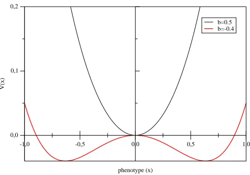
The fluctuating surrounding is modelled with the help of the functionV(x, t) = 1
4x 4+ 1
2b(t)x
2, wherexis representing phenotype and the coefficientb(t) shows the
cos(ωt) time dependence. The closer the value xof an individual to the minimum of
V(x, t) the better adapted its genotype to the surrounding. We observed that the life span of the organisms strongly depends on the value of the frequencyω. It becomes the shorter the often are the changes of the surrounding. However, there is a tendency that the species which have a higher valueaRof the reproduction age win the competition
with the other species.
Another observation is that small evolutionary changes of the inherited genetic information lead to spontaneous bursts of the evolutionary activity when many new species may appear in a short period.
1
Introduction
the various types of the predator-prey systems. They may exhibit many inter-esting features such as chaos (e.g. the recent papers on the topic [3] – [6]) and phase transitions (e.g. [3, 7, 8]). The possible existence of chaos became evident since the work of May [9, 10]. However, usually the studies concerning chaos in biological populations do not contain the discussion of the role of the inher-ited genetic information in it. The discussion of a predator-prey model with genetics has been started by Ray et al. [11], who showed that the system passes from the oscillatory solution of the Lotka-Volterra equations into a steady-state regime, which exhibits some features of self-organized criticality (SOC). Our study [8] on the topic was the Lotka-Volterra dynamics of two competing pop-ulations, prey and predator, with the genetic information inherited according to the Penna model [12] of genetic evolution and we showed that during time evolution, the populations can experience a series of dynamical phase transi-tions which are connected with the different types of the dominant phenotypes present in the populations. Evolution is understoood as the interplay of the two processes: mutation, in which the DNA of the organisms experiences small chemical changes, and selection, through which the better adapted organisms have more offsprings than the others. The problem of speciation from evolution has been studied recently by McManus et al. [13] in terms of a microscopic model. They confirmed that the mutation and selection are sufficient for the appearance of the speciation. We followed their result and in this study we consider a closed ecosystem with a variable number of species competing for the same energy resources. The total energy of the ecosystem cannot exceed the value Ω and every individual costs a respective amount of energy units. We show that the small evolutionary changes of the inherited genetic information result in the bursts of evolutionary activity during which new species appear. Some of the species become better adapted to the fluctuating surrounding and they win the competition for the energy resources.
Our model belongs to the class of Lotka-Volterra systems describing one prey (represented by a self-regenerating energy resources of the ecosystem) and a variable number of the predators competing for the same prey.
2
Evolution of energy resources
All species in the ecosystem under consideration use the same energy resources.
In the model, the number NE(t) of the energy units available for the species
satisfies the differential equation
whereN(t) represents the total number of all individuals in the ecosystem (from
represents relative decrease ofεEcaused by the living organisms. The equation
means that regeneration of the energy resources in the ecosystem takes some time and its speed depends on the number of the living organisms. The above equation also ensures that the size of the species cannot be too big and the number of the species coexisting in the same ecosystem is limited. Otherwise they would exhaust all the energy resources of the ecosystem necessary for life processes.
In the case when N(t) = 0, i.e., if there are no living organisms in the
ecosystem, the Eq.1 reduces to the well known logistic differential equation with the following analytical solution [14]
1
ΩNE(t) =
α
α+ (1−α) exp−εE(t−t0)
, (3)
and the initial condition Eq.2.
We adapt the above solution into our model (Eq.1). To this end we assume that the individuals from all species in the ecosystem under consideration may
reproduce only at discrete time t = 0,1,2,3, . . . (otherwise N(t) = const),
whereasNE(t) remains a continuous function of t between these discrete time
values. Say, if there isN(t0) individuals at the discrete time valuet=t0 then
the value N(t) remains constant (N(t) = N(t0)) in the whole time interval
[t0, t0+ 1). The analytical solution of Eq.1 in this time interval is the following
1
ΩNE(t) =
α
α+ (1−α) exp−εE(1−γENΩ(t))(t−t0)
f or t < t1, (4)
where the initial condition is represented by Eq.2 and t1 = t0+ 1. At time
t =t1 the species reproduce themselves and a new value, N(t1), becomes the
initial condition for the next time interval, [t1, t1 + 1). The numbers N(t)
(t= 0,1,2,3, . . .) result from the computer simulation of mutation and selection applied to the species in the ecosystem according to the Penna model [12] of genetic evolution. The Penna model of evolution represents evolution of bit-strings (genotypes), where the different bit-bit-strings replicate with some rates and they mutate. Hence, in our model we have two types of dynamics, the
continuous one for the numberNE(t) of energy units and the discrete one for
genetic evolution of bit-strings.
3
Species evolution
We restrict ourselves to diploid organisms and we follow the biological species concept that the individuals belonging to different species cannot reproduce themselves, i.e., they represent genetically isolated groups. The populations of each species are characterized by genotype, phenotype and sex. Once the individuals are diploid organisms there are two copies of each gene (alleles) in their genome - one member of each pair is contributed by each parent. In
computer simulations) located in two chromosomes. We agreed that the first
L′ sites in the chromosomes represent the housekeeping genes [15], i.e. the
genes which are necessary during the whole life of every organism. We assumed
that there also exist L−L′ additional ”death genes”, which are switched on
at a specific age a = 1,2, . . . , L−L′ of living individual. The idea of the
chronological genes has been borrowed from the Penna model [12, 16, 17] of biological ageing. The term ”death gene” has been introduced by Cebrat [18] who discussed the biological meaning of the genes which are chronologically switched on in the Penna model. The maximum age of individuals is set to
a=L−L′. It is the same for all species. All species have also the same number
L′ of the housekeeping genes and the same numberL−L′ of the chronological
genes. However, they differ in the reproduction ageaR, i.e., the age at which
the individual can produce the offsprings. The individuals can die earlier due to inherited defective genes. We assume, that it is always the case, when an
individual reaches the ageaand in its history until the ageathere have appeared
three inactive genes in the genotype (inactive gene means two inactive alleles). We make a simplified assumption, that all organisms fulfill the same life functions and each function of an organism (does not matter what species) has been coded with a bit-string consisting of 16 bits generated with the help of a
computer random number generator. We have decided onLdifferent functions
and the corresponding bit-strings represent the patterns for the genes. The genes of all species are represented by bit-strings which differ from the
respec-tive pattern by a Hamming distanceH ≤2. Otherwise the bit-strings do not
represent the genes. In order to distinguish the species, we have introduced the concept of an ideal predecessor, called Eve, who uniquely determines all indi-viduals belonging to the particular species. Namely, the indiindi-viduals have genes
which may differ from the genes of Eve only by a Hamming distance H ≤ 1.
Genes, which differ from the genes of Eve by a Hamming distanceH >1 and,
simultaneously, which differ from the pattern by a Hamming distance H ≤ 2
represent mutated genes. They are potential candidates to contribute to a new species but they are considered as the inactive genes for the species under con-sideration. If there happens another individual with the mutant gene in the same locus then these two mutants can mate (different sex is necessary as well
as the agea≥aR) and they can produce offsrings. In the latter case the new
species is created with Eve who represents Eve of the old species except for the mutant genes. In our computer simulations the new species ususally are extinct due to the mechanism of genetic drift. However, after long periods of ’stasis’ there happen bursts of the new species which are able to live for a few thousands of generations or even more. They also can adapt better to the surrounding and they can dominate other species. The small changes of the inherited genetic information are realized through the point mutations.
A point mutation changes a single bit within the 16-bit-string representation of a gen and according to the above assumptions the gene affected by a mutation
may pass to one of three states: S = 1 (gene specific for the species), S = 2
(mutant gene, potential candidate of a new species),S= 0 (defected gene). In
-1,0 -0,5 0,0 0,5 1,0
Figure 1: Phenotype-surrounding interaction functionV(x, t) = 12x4+1
2b(t)x 2
for two values ofb(t) (0.5 and -0.4).
with probabilityp= 0.1. Hence, there is still a possibility for back mutations.
Genes are mutated only at the stage of the zygote creation - one mutation per individual.
The life cycle of diploids needs an intermediate stage when one of the two copies of each gene is passed from the parent to a haploid gamete. Next, the two gametes produced by parents of different sex unite to form a zygote.
In the model, phenotype is defined as a fractional representation of the 16-bit-string genes, where each gene is translated uniquely into a fractional number
xfrom the interval [−1,1]. The phenotype is coupled with the surrounding with
the help of the functionV(x, t) as follows:
where the fluctuations of the surrounding are represented by the coefficientb(t).
The function V(x, t) has one minimum, x = 0, for b > 0 and two minima,
x=±p
|b|, for b <0 as in Fig.1. We use them to calculate gene quality, q, in
the variable surrounding
q=e−(V(x,t)−Vmin(t))/T, q∈[0,1], (6)
where the parameterT has been introduced to control selection. The smaller
value ofT the stronger selection. Next, we calculate the fitness Q of the
indi-viduals, say at agea, to the surrounding with the help of the average
qi= max {q(1)i δ(S
where the indices (1) and (2) denote, respectively, the first allele and the second
allele at locus i = 1,2, . . . , L′+aand Si = 0,1,2 represent their states. The
symbolsδ() denote Kronecker delta. The inactive alleles and mutant genes do
not contribute toQand alwaysQ∈[0,1].
We decided to determine the amount of possible offsprings by projecting
the fitness of the parents, QF (female) and QM (male), onto the number of
produced zygotes
Nzygote= max{1,10×min(QF, QM)}, (9)
where at least one zygote is produced and the maximum number of zygotes is equal to 10. In the computer simulations, the zygotes are mutated, after they are created, and they can be eliminated if at least one housekeeping gene becomes inactive. The individuals may reproduce themselves after they reach
the age a = aR. The genotypes of the parents who are better adapted to
the surrounding generate more offsprings. The mutants, if they happen (they
posses genes with the Hamming distance H >1 from Eve) cannot mate with
the non-mutants.
We assume that the sex of a diploid individual is determined with the help of a random number generator at the moment when it is born and it is unchanged during its life.
4
Computer algorithm
We investigate the species with respect to speciation. In most computer simula-tions we observed evolving single species and analyzed the offsprings of the new mutant species originating from the old one. The secondary order speciation, i.e., the speciation taken place from the mutant species, has not been consid-ered. However, we investigated the case when initially there are a few species in the ecosystem and the results qualitatively were the same as for single initial species.
In the simulation, it is very important to prepare the genetic information in a proper way. It is obvious that in the evolution process some genes are not nec-essary during the whole life, e.g., they may become important only near the end of life, and it is possible that they could be defective since the individual under consideration was born. Therefore, first we prepare the initial species in the time independent surrounding for a few thousands generations until the inher-ited genetic information is represented by a steady state flow between suceeding generations. Then the distribution of inactive genes becomes time independent. Only after that we switch on the fluctuations of the surrounding, which in our
case are represented by the coefficientb(t) =−1
2−cos(ωt), and all the initially
INITIAL SPECIES PREPARATION:
(1) generateL bit-strings (16 bits) representing life functions of the
or-ganism and which are the patterns for genes
(2) generateNs predecessors (Eve) of the initial species (Hamming
dis-tance of each gene from the respective pattern, H <= 2, and then
S1= 1, S2= 1, . . . SL= 1)
(3) for each Eve, representing the species 1,2, . . . , NsconstructNM males
andNF females (NM =NF) who have each gene at distanceH ≤1
from the corresponding gene of Eve.
(4) evolve separately each species 1,2, . . . , Nsas follows:
(i) increase the age of all individuals by 1
(ii) remove from the population all individuals who should die
be-cause they have exceeded the maximum age (L−L′) or during
their life until now they have collected three inactive ”chrono-logical” genes.
(iii) [optionally] the Verhulst factor is applied, i.e. every
individ-ual survives with the same probability (1−(NM+NF)/Nmax),
where Nmax is the maximum allowed number of individuals in
the population under consideration.
(iV) select at random a female and a male for whom a≥aR and let
them produceNzygotes according to Eq.9.
(V) each zygote is mutated. We assume that the housekeeping genes cannot be inactive. Therefore, at least one defected housekeeping gene kills zygote. The total numer of the zygotes in the
popu-lation which survive cannot exceed the numberεpop(NE/Ω)NR,
where NR is the total number of pairs of individuals, female
and male, whose age a≥aR. The parameter εpop controls the
allowed number of zygotes.
(Vi) Decrease the total number of energy units by the number N(t)
of all individuals (parents and their new-born offsprings), i.e.,
NE(t) =NE(t−1)−N(t)
(Vii) regenerate the ecosystem energy according to Eq.4 (Viii) goto (i) unless the stop criterion is fulfilled
SPECIES IN VARIABLE SURROUNDING:
(5) allNsspecies are put together in the ecosystem.
(6) t=t+ 1
(7) calculateb(t) representing surrounding fluctuation
(8) check all individuals from the old species with respect to mutants
(who have, at least at one locus, k = 1, . . . , L, two bit-strings
rep-resenting the pair of the alleles at stateS(1) = 2 andS(2) = 2). If
create Eve, the pattern of new species, and look for other mutants in the same species consistent with the created Eve. Determine a new
value of the reproduction age aR ∈ [1, L−L′] for the species with
the help of the computer random number generator. Remove new species from the old species.
(9) step (i) from above (10) step (ii) from above (11) step (iii) from above (12) step (iV) from above
(13) step (V) but nowNR concerns all species.
(14) step (Vi), where N(t) concerns all species (15) step (Vii)
(16) goto (6) unless the end of the simulation
5
Results and discussion
Limiting the amount of energy resources in the ecosystem introduces strong selection between the species competing for the resources. In our case the se-lection takes place through limiting the number of the new-born offsprings in the ecosystem. Namely, in the model, their number cannot exceed the value
εpop(NE(t)/Ω)NR, where NR is the number of parents, female and male, from
all species. Thus, the individuals who are better adapted to the environment
(larger value ofQ, Eq.7) dominate other individuals because they produce more
offsprings. In our model, the better adaptation results from the phenotype x
closer to the minimumxmin of the function V(x, t). We could expect that in
a time independent surrounding the mutations decreasing the fitness of the or-ganism lead to its elimination and in result to the elimination of the affected genes. However, in a changing environment the species need an ability to react to new situations. The quality of genes in a fluctuating surrounding is changing, i.e., we cannot tell any more that some genes are bad and some are good. There will be preferred genes which adapt better to the changes.
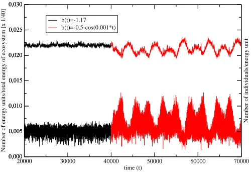
In Fig.2, we show the effect of the changing environment on the old
pop-ulation (aR = 5, L = 16, L′ = 5), which was aging in a time independent
surrounding through 40000 generations. The changing enviroment is modelled
with the help of the coefficient b(t) in the function V(x, t) (Eq.5). We have
chosen
b(t) =−1
2 −cos(ωt), (10)
where ω denotes the frequency of the environment changes. We should take
20000 30000 40000 50000 60000 70000
Number of energy units/total energy of ecosystem [x 1/40]
b(t)=-1.17 b(t)=-0.5-cos(0.001*t)
Figure 2: The effect of the transition from the time independent surrounding (b(t) =−1.17,t <40000) to the one varying in time (b(t) =−12−cos(0.001t),
t ≥ 40000) on the size of the single species (aR = 5, amax = 11) and on the
number of the energy units available for the species. The bottoom curve follows the size changes of the species whereas the upper curve shows the corresponding energy changes in the ecosystem.
with the species as the predator and the energy as the prey. Once the fluctuating
environment changes fitnessQ of all individuals, the number of the new-born
offsprings follows the environment fluctuations and in consequence there appear the energy oscillations. Notice, that in a changing environment the size of the population under consideration undergoes much stronger fluctuations than in the time-independent case. It is connected with the changes of the inherited genetic information.
In Fig.3 we have presented the age profiles of the fraction of the inactive ”chronological” genes in the population from Fig.2. The profiles concerning the
generations att= 20000 and t= 40000 refer to time independent surrounding.
Although we have introduced in the model the back mutations for the inactive genes (the bit-strings corresponding to inactive genes may mutate into another
bit-string with probabilityρ= 0.1) we can observe that, while time is
increas-ing, the shape of the profiles tends to the one which is time independent. It determines the average life span of individuals which is ranging from the age
a= 1 toa= 7. On the other hand, the profiles corresponding to time dependent
environment show both shrinking and enlarging of the life span. Effectively, the population becomes much younger than during its previous evolution in the time independent surrounding. More frequent fluctuations of the surrounding make this effect even stronger. It is evident from Fig.4 where the same old species, under consideration, experiences the surrounding changing with the higher
fre-quency ω = 0.01. We can observe that the effect of the frequently changing
1 2 3 4 5 6 7 8 9 10 11 genotype site specific for age a
0 0,2 0,4 0,6 0,8 1
fraction of defected genes specific for age a
t=20000 t=40000 t=50000 t=100000 t=140000
Figure 3: The effect of the change of the time independent surrounding to
the one varying in time, at t ≥ 40000, on the distribution of the defected
”chronological” genes for the situation presented in Fig.2.
1 2 3 4 5 6 7 8 9 10 11
genotype site specific for age a 0
0,2 0,4 0,6 0,8 1
fraction of defected genes specific for age a
t=20000 t=40000 t=50000 t=100000 t=140000
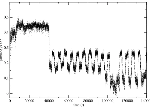
0 20000 40000 60000 80000 100000 120000 140000
Figure 5: The phenotype evolution for the situation presented in Fig.2.
All our simulation were done with a constant mutation rate (one mutation per genome) and we did not discuss the effect of the various values of the mutation rate on the above results.
The evolution of the average phenotype of the species from the example in Fig.2 has been shown in Fig.5. The same data, but presented with the help of a histogram have been shown in Fig.6.
Notice, that there is a trend to minimize the environment fluctuations and the genes, which were well adapted in the time independent environment, do not have the ability to follow the environment fluctuations. They can be even eliminated from the genetic bank of the species if the fluctuations become more frequent.
The environmental changes influence the size of all species in the ecosystem end this is the reason that some of them may be eliminated. The regeneration of the energy resources in the ecosystem takes some time and too rapid a growth of some species, e.g., mutant species, acts as a sudden cataclysm for the other species. The Lotka-Volterra systems have a self-regulatory character and there exist threshold values for the fraction of destroyed population above which the system returns to its previous state ([19],[8]). However, in the case of genetic populations, if the catastrophe is applied for many generations, one can observe that the age profile of the fraction of defective genes in the population may loose its stability and next the species becomes extincted ([8]). Thus the appearance of the new species, even for a relatively short period, can eliminate the old species.
In our computer simulations we associate a new value,aR, of the
0 0,1 0,2 0,3 0,4
Figure 6: The histogram of the average usage of the phenotypexin the
evolv-ing species (from Fig.2) when there is time independent surroundevolv-ing (r.h.m histogram), and when there is fluctuationg environment.
that the events, representing the appearance of the new species with the small
valueaR (aR ∼ 1), are usually represented by short duration ”bursts” of the
population size and they vanish as rapidly as they have appeared. In the exam-ple from Fig.7 the are represented by the highest blobs painted in black, at the bottoom of the figure. It is easy to explain the phenomenon, as in this case the life span of individuals practically is shrinking to the activity of single gene and the individuals die after they reproduce themselves. The active genes cannot effectively adapt to the changing environment. How important the range of life span for species stability is, can be also concluded from the histograms in Fig.8.
There are presented histograms of the average usage of the phenotypexof
the species representing the predecessor (aR = 5) and two descendant species
(aR = 2,7). It is evident that the average value x representing the species
with aR = 2 oscillates far away from the optimum values (variable minima
of V(x, t)), because there is an insufficient number of genes adapted to the
variable surrounding. The situation is a little bit better with the predecessor (old species). However, it is evident that it cannot be stable over a long time
in a variable surrounding. The most stable species is the one for whichaR= 7,
because in its population there are inherited genes which have adapted to the
variable surrounding (the range ofxis almost symmetric with respect tox= 0).
0 5000 10000 15000 20000
Number of energy units/Total energy
0,0
Number of individuals/energy unit [ x 25]
Figure 7: The effect of the speciation from the old species (earlier aging for
40000 generations in time independent environment) in a fluctuating
environ-ment (b(t) = −12 −cos(0.01t) on the evolution of the energy resources. In
the bottom part of the figure there have been shown a few examples of the new species created in the course of the evolution. The energy cost of the new species creation or extinction is reflected by the terrace-like changes in the upper curve. The survived species have not been shown for clarity of the picture.
-0,2 0 0,2 0,4
normalized number of events with phenotype (x)
aR=5, OLD aR=7, MUTANT aR=2, MUTANT
Figure 8: Histograms of the phenotype usage in the environment changing with
the frequencyω= 0.02 in the case of three species: the predecessor population
(aR = 5), and two descendant populations (aR = 7,aR = 2). The frequency of
6
Conclusions
We have discussed a model of species evolution in an ecosystem where the en-ergy resources regenerate themselves according to a logistic differential equation. The model belongs to the class of the Lotka-Volterra systems where the energy resources represent prey and the species represent predator. The number of the species present in the ecosystem under consideration results from evolution, which is understoood as the interplay of the two processes only, mutation and selection. We observed that after long periods of ’stasis’ there happen bursts of the new species which are able to live for thousands of generations. We have observed that in a variable surrounding the species, for which the reproduction
ageaRis too small, they are very unstable even if their size substantially exceeds
the size of the populations specific for other species. In our model, they usually cause the elimination of other species. Simultaneously, the resulting increase in the energy resources makes the next speciations possible.
References
[1] V. Volterra,Th´eorie math´ematique de la lutte pour la vie, Gauthier-Villars,
Paris 1931
[2] L.E. Reichl,A Modern Course in Statistical Physics, Edward Arnold
(Pub-lishers) 1980, pp. 641-644
[3] R. Gerami and M.R. Ejtehadi, Eur. Phys. J. B13, 601 (2000)
[4] B.E. Kendall, Chaos, Solitons and Fractals12, 321 (2001)
[5] V. Rai, W.M. Schaffer, Chaos, Solitons and Fractals 12, 197-203 (2001) [6] J. Vandermeer, Lewi Stone, B. Blasius, Chaos, Solitons and Fractals 12,
265-276 (2001)
[7] A.F. Rozenfeld, E.V. Albano, Physica A266322 (1999)
[8] A. Duda, P. Dy´s, A. Nowicka, M.R. Dudek, Int. J. Mod. Phys. C11,
1527-1538 (2000)
[9] R.M. May, Science186, 645-647 (1974)
[10] R.M. May, Nature216, 459-467 (1976)
[11] T.S. Ray, L. Moseley, N. Jan, Int. J. Mod. Phys. C9, 701 (1998)
[12] T.J.P. Penna,J. Stat. Phys.78: 1629 (1995)
[13] S. MCManus, D.L. Hunter, and N. Jan, T. Ray, L. Moseley, Int. J. Mod.
Phys. C10, 1295-1302 (1999)
[14] J.H.E. Cartwright and O. Piro, Int. J. Bifurc. Chaos2, 427-449 (1992)
[15] E. Niewczas, A. Kurdziel, and S. Cebrat, Int. J. Mod. Phys. C 11, 775
(2000)
[16] T.J.P. Penna and D. Stauffer, Int. J. Mod. Phys. C6, 233 (1995)
[17] Moss de Oliveira,S., P.M.C. de Oliveira
and D. Stauffer. 1999. Evolution, Money, War, and Computers, Teubner,
Stuttgart-Leipzig
[18] S. Cebrat, Physica A258, 493 (1998)
[19] A. P¸ekalski and D. Stauffer, Int. J. Mod. Phys. C9, 777 (1998)
[20] P.Bak, K. Sneppen, Phys. Rev. lett.71, 4083 (1993)
[21] K. Sneppen, Physica A221, 168-179 (1995)