Brain lesion segmentation from diffusion weighted MRI based on adaptive thresholding and gray level co-occurrence matrix.

(1)

ISSN: 2180 - 1843 Vol. 3 No. 2 July-December 2011

Brain Lesion Segmentation from Difusion-weighted MRI based on Adaptive Thresholding and Gray Level Co-occurrence Matrix

1

Abstract

This project presents brain lesion segmentation of difusion-weighted magnetic resonance images (DWI) based on thresholding technique and gray level co-occurrence matrix (GLCM). The lesions are hyperintense lesion from tumour, acute infarction, haemorrhage and abscess, and hypointense lesion from chronic infarction and haemorrhage. Pre-processing is applied to the DWI for intensity normalization, background removal and intensity enhancement. Then, the lesions are segmented by using two diferent methods which are thresholding technique and GLCM. For the thresholding technique, image histogram is calculated at each region to ind the maximum number of pixels for each intensity level. The optimal threshold is determined by comparing normal and lesion regions. Conversely, GLCM is computed to segment the lesions. Diferent peaks from the GLCM cross-section indicate the present of normal brain region, cerebral spinal luid (CSF), hyperintense or hypointense lesions. Minimum and maximum threshold values are computed from the GLCM cross-section. Region and boundary information from the GLCM are introduced as the statistical features for segmentation of hyperintense and hypointense lesions. The proposed technique has been validated by using area overlap (AO), false positive rate (FPR), false negative rate (FNR), misclassiied area

Brain Lesion segmentation from

Diffusion-weighteD mri BaseD on aDaptive threshoLDing anD

gray LeveL Co-oCCurrenCe matrix

norhashimah mohd saad

1

, s.a.r. abu-Bakar

2

, abdul rahim abdullah

3

,

Lizawati salahuddin

1

, sobri muda

4

, musa mokji

2

1

Faculty of Electronics & Computer Engineering,

Universiti Teknikal Malaysia Melaka, Malaysia

2

Faculty of Electrical Engineering, Universiti Teknologi Malaysia, Malaysia

3

Faculty of Electrical Engineering, Universiti Teknikal Malaysia Melaka,

Malaysia

4

Radiology Department, Medical Centre, Universiti Kebangsaan Malaysia,

Malaysia

Email:

1

norhashimah@utem.edu.my,

2

syed@ke.utm.my,

3

abdulr@utem.edu.my,

1

lizawati@utem.edu.my,

4

sobri_muda@yahoo.com,

3

musa@ke.utm.my

(MA), mean absolute percentage error (MAPE) and pixels absolute error ratio (r_err). The results are demonstrated in three indexes MA, MAPE and rerr, where 0.3167, 0.1440 and 0.0205 for

GLCM, while 0.3211, 0.1524 and 0.0377 for thresholding technique. Overall, GLCM provides beter segmentation performance compared to thresholding technique.

Keywords: DWI, GLCM, segmentation, thresholding.

i. introDuCtion

Tumor, infarction (stroke/ischemia), haemorrhage (bleeding/ ischemia) and infection (abscess) are the example of brain lesions that are afected in the brain cerebrum. In 2006, it was reported that tumor and brain diseases such as brain infarction and haemorrhage were the third and fourth leading cause of death in Malaysia [1]. The incidence of brain tumor in 2006 was 3.9 among males and 3.2 among females per 100,000 populations with a total of 664 cases reported by the

(2)

ISSN: 2180 - 1843 Vol. 3 No. 2 July-December 2011 Journal of Telecommunication, Electronic and Computer Engineering

2

Minister of Health Malaysia. In the United States, the combined incidence of primary brain tumor was 6.6 per 100,000 persons per year with a total of 22,070 new cases in 2009 [2], while brain infarction afects approximately 750,000 new cases per year [3].

Interpretation of brain imaging plays an important part in diagnosis of various diseases and injury. Magnetic resonance imaging (MRI) is one of the popular, painless, non-radiation and non-invasive brain imaging techniques. Nevertheless, assessment of brain lesion in MRI is a complicated process and typically performed by experienced neuroradiologists. An expert neuroradiologist performs this task with a signiicant degree of precision and accuracy. It can oten be diicult for clinicians to precisely assess the lesion on the basis of radiographic appearance. Therefore, quantitative analysis using computers can help radiologists to overcome these problems. Due to the importance of brain imaging interpretation, signiicance research eforts have been devoted for developing beter and more eicient techniques in several related areas including processing, modeling and understanding of brain images [4].

Over the past several years, developments in MRI unit have enabled the acquisition of MR imaging using fast and advanced techniques, proving extremely useful in various clinical and research applications such as difusion-weighted MRI (DW-MRI or DWI) [5]. DWI proicient to provide image contrast that is dependent on the molecular motion of water, which can alter by disease [6]. The image is bright (hyperintense) when the rate of water difusion in the cell membrane is restricted and dark (hypointense) when the difusion is elevated [6]. DWI provides very good lesion contrast compared to the appearance in conventional MRI [3]. Research have shown DWI is considered as the most sensitive technique in detecting early acute neurological

disorders, stroke, infection, trauma and tumor [3,6-7].

Segmentation or separation of speciic region of interest (ROI) of pathological abnormalities from MR images is an essential process for diagnosis and treatment planning. Accurate segmentation is still a challenging task because of the variety of the possible shapes, locations and image intensities of various types of problems and protocols. Computerized segmentation process is essential to overcome these problems. A large number of approaches have been proposed by various researchers to deal with various MRI protocols [8]. These approaches were introduced to solve the problems of automatic lesion detection and segmentation in various conventional MRI.

Thresholding based segmentation discriminates pixels according to their gray level value. The key parameter in the thresholding process is the choice of the threshold value. In this study, histogram thresholding is applied to separate hyperintense lesion from DW images. The rationale being that the brightness of hyperintense lesion pixels are higher than the normal pixels.

(3)

3 Beside the widely known thresholding,

this paper proposes a new statistical information based on region and boundary information from the GLCM. The analysis involves both thresholding and GLCM computation to pre-processed DWI; calculating the minimum and maximum threshold values from GLCM cross-section; and segmenting the hyperintense or hypointense lesions based on thresholding and region and boundary information from the GLCM. Segmentation evaluation is made in order to analyze the performance of the proposed techniques.

ii. Diffusion-weighteD mri

a. Brain Lesion

(a) Normal (b) Solid tumor (c) Acute infarction

(d) Abscess (e) Haemorrhage (f) Chronic infarction

Fig. 1 Original DWI with brain lesion indicated by a white circle Fig. 1 Original DWI with brain lesion indicated by a white circle

Fig. 1 shows DWI intensities in major brain lesion, where the lesion is indicated by a white circle. In normal brain, the region consists of brain tissue (normally called as gray and white mater tissue in conventional MRI) and a cavity which is full of cerebral spinal luid (CSF) located in the middle of the brain, as shown in Fig. 1(a). The DWI intensity for CSF is dark. Fig. 1 (b-f) shows several brain lesions, in which the intensity can be divided into hyperintense and hypointense.

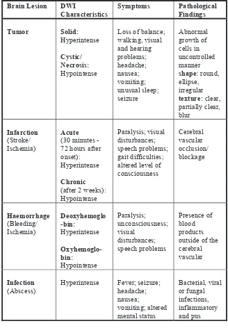
DWI hyperintense lesion includes acute infarction, acute haemorrhage, solid tumor and abscess. Chronic infarction and necrosis tumor appear to be hypointense in DWI. The summary of major brain lesions, types, symptoms and

pathological indings is summarized in Table I. Nevertheless, this paper is only focused on the hyperintense lesions. Based on our hypothesis, the hyperintense lesions in DWI can be well separated from the normal tissue because of its high gray level intensity.

Table 1 Description of brain lesions, types,

symptoms and pathological indings [25-28] and

ogical e classical

features s to analyze rious MR

tically I is paper

and volves rocessed reshold ng the g and e GLCM.

ze the

B. Imaging Parameter

Brain Lesion DWI Characteristics

Symptoms Pathological Findings

Tumor Solid:

Hyperintense

Cystic/ Necrosis:

Hypointense

Loss of balance; walking, visual and hearing problems; headache; nausea; vomiting; unusual sleep; seizure

Abnormal growth of cells in uncontrolled manner

shape: round, ellipse, irregular

texture: clear, partially clear, blur

Infarction

(Stroke/ Ischemia)

Acute

(30 minutes - 72 hours after onset): Hyperintense

Chronic

(after 2 weeks): Hypointense

Paralysis; visual disturbances; speech problems; gait difficulties; altered level of consciousness

Cerebral vascular occlusion/ blockage

Haemorrhage

(Bleeding/ Ischemia)

Deoxyhemoglo -bin:

Hyperintense

Oxyhemoglo-bin:

Hypointense

Paralysis; unconsciousness; visual disturbances; speech problems

Presence of blood products outside of the cerebral vascular

Infection

(Abscess)

Hyperintense Fever; seizure; headache; nausea; vomiting; altered mental status

Bacterial, viral or fungal infections, inflammatory and pus

B. imaging parameter

(4)

4

iii. proposeD teChniQues

a. thresholding technique

The lowchart of the proposed segmentation is shown in Fig. 2. The samples of brain DWI dataset are irst collected. In the pre-processing stage, several algorithms are applied to enhance the images. The intensity is normalized from 0 to 1, the background and skull are removed and then the intensity is enhanced using two diferent algorithms which are gamma-law transformation and contrast stretching. The algorithms are applied to span the narrow range of DWI histogram for thresholding purpose. The segmentation process starts at full image and splits to 8 x 8 regions. The lesion intensity range is analysed based on thresholding technique. This is done by calculating image histogram at each region and inding the maximum number of pixels at each intensity level. An optimal threshold is determined by comparing normal and lesion regions in the histogram. Region of interest (ROI) is then segmented based on the optimal threshold.

Fig. 2 Flowchart of the proposed thresholding technique

φ φ ≤ ≤ ≤ ≤ φ ≤ ≤ _φ

∑∑

_{= =}_⎩⎨⎧ = = = φ φ φ ⎪ ⎪ ⎩ ⎪ ⎪ ⎨ ⎧ = = = ± = ± = φ φ φ φ m m m m φ φ φ φ φ φ φ ⎪ ⎪ ⎩ ⎪ ⎪ ⎨ ⎧ = − − = − = + − = + = φ φ φ φ φ

(

+ + +

)

= Preprocessing Segmentation

DWI Brain Image

Image Normalization

Background Removal

Image Enhancement

Image Splitting

(Block Processing)

Histogram

Thresholding

Fig. 2 Flowchart of the proposed thresholding technique

B. gLCm

GLCM [17, 29] is a matrix of relative frequencies in which two neighbouring pixels separated by distance d, at angular orientation φ, occur in an image. One pixel is with gray level u and the other is with gray level v. The angular orientation φ is quantized to four directions which are horizontal, diagonal, vertical and of-diagonal, or 0o_{, 45}o_{, 90o and 135}o_, respectively. For an image I(x,y), where the image has 1≤x≤N_x pixels in horizontal direction and 1≤y≤ N_y pixels in vertical direction. Suppose that the image has Ng resolution levels in which u represents the gray level of pixel I(x,y) and v represents the gray level of the nearest-neighbour pixel where 0≤u,v≤N_g-1. The GLCM,

φ

≤ ≤ ≤ ≤

ay level of the nearest-neigh _φ

≤ ≤ The GLCM, G(u,v)d,_φ is

∑∑

(

+ + +

)

=

is calculated as:

at. own in llected. φ φ ≤ ≤ ≤ ≤ φ ≤ ≤ _φ

∑∑

_{= =}_⎩⎨⎧ = =

=Nx y x N y d d v v y x I u v u G 1 1 , , otherwise 0 and ) , ( if 1 ) , ( _φ φ φ

v is referred to the nearest neighbour pixel, defined

⎪ ⎪ ⎩ ⎪ ⎪ ⎨ ⎧ = = = ± = ± = φ φ φ φ m m m m φ φ φ φ φ φ φ ⎪ ⎪ ⎩ ⎪ ⎪ ⎨ ⎧ = − − = − = + − = + = φ φ φ φ φ

(

+ + +

)

= φ φ ≤ ≤ ≤ ≤ φ ≤ ≤ _φ

∑∑

_{= =}_⎩⎨⎧ = = = φ φ (1)

φ defined as:

(

+ + +

)

= llected. s are applied to

0 to 1,

φ φ ≤ ≤ ≤ ≤ φ ≤ ≤ _φ

∑∑

_{= =}_⎩⎨⎧ = = = φ φ φ , d

v is refe

(

+ + +

)

=

is referred to the nearest neighbour pixel, deined as:

φ φ ≤ ≤ ≤ ≤ φ ≤ ≤ _φ

∑∑

= =⎩⎨ ⎧ = = = φ φ φ ⎪ ⎪ ⎩ ⎪ ⎪ ⎨ ⎧ = = = ± = ± = o o o o d φ d y d x I φ y d x I φ d y d x I φ d y x I v 135 ) , ( 90 ) , ( 45 ) , ( 0 for ) , ( , m m m m φ (2) d φ φ φ φ φ φ ⎪ ⎪ ⎩ ⎪ ⎪ ⎨ ⎧ = − − = − = + − = + = φ φ φ φ φ

(

+ + +

)

= (2)

For d=1, the eight nearest-neighbour orientation of φ corresponding to pixel I(x,y) can be illustrated in Fig. 3.

φ φ ≤ ≤ ≤ ≤ φ ≤ ≤ _φ

∑∑

_{= =}_⎩⎨⎧ = = = φ φ φ ⎪ ⎪ ⎩ ⎪ ⎪ ⎨ ⎧ = = = ± = ± = φ φ φ φ m m m m φ φ

3 Eight nearest-neighbour pixel cells to pixel *.

φ φ φ φ φ ⎪ ⎪ ⎩ ⎪ ⎪ ⎨ ⎧ = − − = − = + − = + = φ φ φ φ φ

(

+ + +

)

=

Fig. 3 Eight nearest-neighbour pixel cells to

pixel *. With d=1; 1 and 5 areφ = 0o_{, 4 and 8}

are φ = 45o_{, 3 and 7 are}φ_{= 90}o_{, 2 and 6 are}φ₌

135o_{. * is the reference pixel I(x,y) [17].}

One of the characteristic of the GLCM is it is diagonally symmetry. Thus, the corresponding adjacent pixel_{s are applied to}llected.

0 to 1,

φ φ ≤ ≤ ≤ ≤ φ ≤ ≤ _φ

∑∑

_{= =}_⎩⎨⎧ = = = φ φ φ , d

v is refe

(5)

Brain Lesion Segmentation from Difusion-weighted MRI based on Adaptive Thresholding and Gray Level Co-occurrence Matrix 5 φ φ ≤ ≤ ≤ ≤ φ ≤ ≤ _φ

∑∑

_{= =}_⎩⎨⎧ = = = φ φ φ ⎪ ⎪ ⎩ ⎪ ⎪ ⎨ ⎧ = = = ± = ± = φ φ φ φ m m m m φ φ φ φ φ φ φ

in equation (2) can be simplified as:

⎪ ⎪ ⎩ ⎪ ⎪ ⎨ ⎧ = − − = − = + − = + = o o o o d φ d y d x I φ y d x I φ d y d x I φ d y x I v 135 ) , ( 90 ) , ( 45 ) , ( 0 for ) , ( ,φ

(3)

In practice, for each d, the matrices for the four orientations

(

+ + +

)

=

_{In practice, for each}_d_{, the matrices for the} four orientations are averaged. Thus, the averaged GLCM, φ φ ≤ ≤ ≤ ≤ φ ≤ ≤ _φ

∑∑

= =⎩⎨ ⎧ = = = φ φ φ ⎪ ⎪ ⎩ ⎪ ⎪ ⎨ ⎧ = = = ± = ± = φ φ φ φ m m m m φ φ φ φ φ φ φ ⎪ ⎪ ⎩ ⎪ ⎪ ⎨ ⎧ = − − = − = + − = + = φ φ φ φ φ

matrices for the four or eraged GLCM, G(u,v) is

(

+ + +

)

=

is computed as:

which , at angular φ φ ≤ ≤ ≤ ≤ φ ≤ ≤ _φ

∑∑

(

Guv_d o Guv_d o Guv_d o Guv_d o

)

v u

G (,)_,₀ (, )_,₄₅ (, )_,₉₀ (,)_,₁₃₅ 4 1 ) , ( = + + + IV. φ φ ≤ ≤ ≤ ≤ φ ≤ ≤ _φ

∑∑

= =⎩⎨ ⎧ = = = φ φ φ ⎪ ⎪ ⎩ ⎪ ⎪ ⎨ ⎧ = = = ± = ± = φ φ φ φ m m m m φ φ φ φ φ φ φ ⎪ ⎪ ⎩ ⎪ ⎪ ⎨ ⎧ = − − = − = + − = + = φ φ φ φ φ

(

+ + +

)

= (4)

iv. image preproCessing

Several Several pre-processing algorithms are applied to DW images for intensity normalization, background removal and intensity enhancement. The original DWI has 12-bit intensity depth unsigned integer. In normalization process, the type of the intensity depth is converted to double precision, where the minimum value is set to 0 while for the maximum is to 1. The DWI includes background image which needs to be removed. This is because the background shares similar gray level values with certain brain structures. The technique for background removal can be found in [30]. Then, image enhancements are applied. Two diferent techniques are used, which are Gamma-law transformation algorithm and contrast stretching. The objective is to evaluate image enhancement that can provide beter segmentation results for thresholding technique.

Gamma-law transformation algorithm is chosen to expand the narrow range of low input gray level values of DWI to a wider range. It has the basic form of s=crγ, where c is amplitude, and γ is a constant power of input gray level, r [31]. γ=0.4 has been found to be the best value based on experiments to enhance the output histogram [32]. The Gamma-law transformation response is shown in Fig. 4.

γ γ

γ

0 0.2 0.4 0.6 0.8

Fig. 4 Image response for gamma-law transformation

= Maximum pixels distributions

Fig. 4 Image response for gamma-law transformation

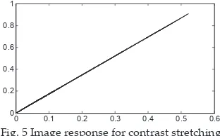
On the other hand, contrast stretching is applied to improve an image by stretching the range of intensity values. Unlike histogram equalization, contrast stretching is restricted to a linear mapping of input to output values. For each pixel, the input gray level, r_{is mapped to}

output, s_{according to equation (5).}

s = ratio * r₍₅₎

where ratio is:

Background Image e Standardiz Background Image Original =

ratio (6)

Standardize Image Background = 0.02 is adopted for this experiment. This value is chosen to correct the image background in-homogeneity. Thus, the images will have similar background value, with the average of 0.02.

γ γ

γ

=

0 0.1 0.2 0.3 0.4 0.5 0.6

0 0.2 0.4 0.6 0.8 1

Fig. 5 Image response for contrast stretching

(6)

6

image histogram. The maximum peak is located at 0.1. Ater applying Gamma-law transformation algorithm, the histogram has been enhanced in which the peak is located at 0.4 as shown in Fig. 6(c). On the other hand, the maximum peak is located at 0.2 for contrast stretching as shown Fig. 6(d).

γ

γ vel, r

γ sed on

The prove es. Unlike to a xel, the ation (5) = (6) r this mage es will have

00 0.1 0.2 0.3 0.4 0.5 0.6 1000 2000 3000 4000 5000 6000 7000

(a) Image and histogram of intensity normalization

00 0.1 0.2 0.3 0.4 0.5 0.6 100 200 300 400 500

(b) Image and histogram of background removal

0₀ _0.2 _0.4 _0.6 _0.8 50 100 150 200 250

(c) Image and histogram of Gamma-law transformation

00 0.2 0.4 0.6 0.8 50 100 150 200 250

(d) Image and histogram of contrast stretching

Fig. 6 Pre-processing steps Fig. 6 Pre-processing steps

v. segmentation proCess

using threshoLDing

teChniQue

For the image segmentation process, irstly the entire image is divided by 8 x 8 regions where 256 x 256 pixels of the entire image is split to 16 x 16 pixels size in each region. Fig. 7 shows the image spliting (block processing) with 16 x 16 pixels size per segment.

1 2 3 4 5 6 7 8

9 10 11 12 13 14 15 16

17 18 19 20 21 22 23 24

25 26 27 28 29 30 31 32

33 34 35 36 37 38 39 40

41 42 43 44 45 46 47 48

49 50 51 52 53 54 55 56

57 58 59 60 61 62 63 64

Fig. 7 Image splitting (16 x 16 pixels size per segment)

= ⎩⎨ ⎧ ≥ =

Fig. 7 Image spliting (16 x 16 pixels size per

segment)

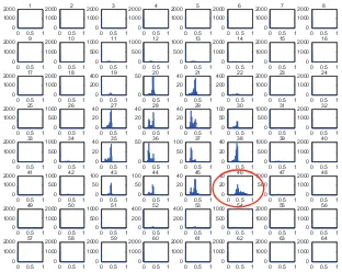
Region 46 which is indicated by red circle is the lesion, examine by neuroradiologist. Next, histogram is calculated at each region as shown in Fig. 8. The red circle shows the histogram distribution of lesion, whereas the others are histogram of normal brain area.

00.5 1 0 1000 2000 1

00.51 0 1000 2000 2

00.51 0 1000 2000 3

00.5 1 0 1000 2000 4

00.5 1 0 1000 2000 5

00.51 0 1000 2000 6

00.51 0 1000 2000 7

00.51 0 1000 2000 8

00.5 1 0 1000 2000 9

00.51 0 1000 2000 10

00.51 0 500 1000 11

00.5 1 0 500 1000 12

00.5 1 0 500 1000 13

00.51 0 1000 2000 14

00.51 0 1000 2000 15

00.51 0 1000 2000 16

00.5 1 0 1000 2000 17

00.51 0 1000 2000 18

00.51 0 200 400 19

00.5 1 0 50 20

00.5 1 0 20 40 21

00.51 0 200 400 22

00.51 0 1000 2000 23

00.51 0 1000 2000 24

00.5 1 0 1000 2000 25

00.51 0 500 1000 26

00.51 0 20 40 27

00.5 1 0 20 40 28

00.5 1 0 20 40 29

00.51 0 50 100 30

00.51 0 500 1000 31

00.51 0 1000 2000 32

00.5 1 0 1000 2000 33

00.51 0 500 1000 34

00.51 0 20 40 35

00.5 1 0 50 36

00.5 1 0 50 100 37

00.51 0 20 40 38

00.51 0 500 1000 39

00.51 0 1000 2000 40

00.5 1 0 1000 2000 41

00.51 0 500 1000 42

00.51 0 50 100 43

00.5 1 0 50 100 44

00.5 1 0 20 40 45

00.51 0 20 40 46

00.51 0 500 1000 47

00.51 0 1000 2000 48

00.5 1 0 1000 2000 49

00.51 0 1000 2000 50

00.51 0 500 1000 51

00.5 1 0 200 400 52

00.5 1 0 200 400 53

00.51 0 500 1000 54

00.51 0 1000 2000 55

00.51 0 1000 2000 56

00.5 1 0 1000 2000 57

00.51 0 1000 2000 58

00.51 0 1000 2000 59

00.5 1 0 1000 2000 60

00.5 1 0 1000 2000 61

00.51 0 1000 2000 62

00.51 0 1000 2000 63

00.51 0 1000 2000 64

Fig. 8 Histogram distribution of each region

= ⎩⎨ ⎧ ≥ =

Fig. 8 Histogram distribution of each region Two histograms which are normal and abnormal (lesion) are then generated. All normal and abnormal regions are overlap respectively to ind the maximum number of pixels at each intensity level. The maximum number of pixels is calculated by using the function shown in equation (7). n)) , m R : 1 (R Max(Pixels Pixels(n)

Max =

Where n is the intensity at level n, R1 and Rm are

⎩⎨ ⎧ ≥ =

= (7)

are regions in

⎩⎨ ⎧ ≥ =

(7)

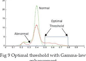
7 for each block is to enhance the lesion

for comparison with normal. This will produce a new histogram as shown in Fig. 9. The optimal threshold is determined by the ROI indicator, which the intensity level of normal histogram is reached zero pixels.

=

0 0.1 0.2 0.3 0.4 0.5 0.6 0.7 0.8 0.9 1 0

5 10 15 20 25

Fig 9 Optimal threshold with Gamma-law enhancement

⎩⎨

⎧ ≥

=

Optimal

Threshold Normal

Abnormal

Fig 9 Optimal threshold with Gamma-law enhancement

Fig. 10 shows the maximum block histogram, which is done by overlapping the histogram in all blocks including both normal and abnormal. By using the proposed technique, we can clearly characterize the lesion area because it has been enhanced.

sion, d at the are

=

0 0.1 0.2 0.3 0.4 0.5 0.6 0.7 0.8 0.9 1 0

5 10 15 20 25

Fig 10 Maximum block histogram

⎩⎨

⎧ ≥

=

Lesion

Fig 10 Maximum block histogram The statistical features representing the hyperintense and hypointense regions are then calculated according to equation (8), where T_optimal is the threshold value to obtain the segmentation.

=

I(x,y)hyperintense=⎧_⎩⎨1₀ for _elsewhereI(x,y)≥Toptimal

=

⎩⎨

⎧ ≥

= (8)

vi. segmentation proCess

using gLCm

Fig. 11 shows an example of GLCM for image in Fig. 1(c). The image has hyperintense lesion due to acute infarction. The GLCM is computed for Ng=128, d=1 and at average orientations, and is represented in a contour plot. Colour intensity represents the co-occurrence frequencies, or the number of repetitions between each pixel pair, u and v. It can be seen that hypointense region and CSF occur at smaller co-occurrence entry; normal brain tissue is located in the middle of the matrix, while hyperintense region exists at higher entry. The red dash-line shows a cross-section at u=v. At this line, the co-occurrence frequency is the highest. The plot also shows that the co-occurrence frequencies are diagonally symmetry and the gray level resolutions are brighter when the co-occurrence transitions increase of-diagonally with the matrix.

Averaged GLCM contour plot

gray level,v

g

ra

y

l

e

v

e

l,

u

20 40 60 80 100

20 30 40 50 60 70 80 90 100

500 1000 1500 2000 2500

Fig. 11 GLCM for DWI in Fig. 1(c)

⎩ ⎨

⎧ ≥ ≥

=

⎩ ⎨

⎧ ≤ ≤

=

≤ ≤ ≤ ≤ ≤ ≤

∑∑

_{= =}_⎩⎨⎧ > =

+ +

+ =

φ

= > + = = Hypointense

region

Normal brain tissue

Hyperintense

region

T

T1 T1

T2

1

2

3

1, 2 1, 3

3, 2

3, 1 2, 1

2, 3

Fig. 11 GLCM for DWI in Fig. 1(c)

a. minimum and maximum threshold

The GLCM G(u,v) is basically shows a representation of a second-order histogram in which the (u,v)th_element is the frequency that pixel pair u co-occurs with v. GLCM cross-section can be constructed in which each entry at u=v is ploted versus the frequency. Fig. 12 shows the GLCM cross-section from the contour plot in Fig. 11.

(8)

8

by very small peaks at the smaller and higher entry, respectively. The magnitudes of the peaks depend on the size of lesions. To ind the minimum and maximum threshold values, the gradient function, or the divergence slope is calculated. The gradient reach maximum when the GLCM frequency is the greatest rate of change, and vice versa. The minimum and maximum threshold (T1 and T2) is set at the irst zero-gradient before and ater the maximum peak, respectively.

respectively.

0 20 40 60 80 100

-400 -200 0 200 400 600 800

1000 Divergence of smooth GLCM

co-occurrence u=v fr e q u e n c y

Fig. 12 GLCM Cross-section and the divergence slope to

⎩ ⎨ ⎧ ≥ ≥ = ⎩ ⎨ ⎧ ≤ ≤ = ≤ ≤ ≤ ≤ ≤ ≤

∑∑

_{= =}_⎩⎨⎧ > = + + + = φ = > + == Min threshold,

T1

Max Threshold,

T2

Max Peak

T1 T1 T2 T2 1 2 3 1, 2 1, 3 3, 2 3, 1 2, 1 2, 3

Fig. 12 GLCM Cross-section and the divergence slope to determine the minimum

and maximum threshold values B. region and Boundary information

from gLCm

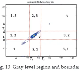
In this research, the region and boundary information are based on the partition of nine regions, which are separated by the minimum and maximum threshold values, T₁ and T₂. Referring to Fig. 13, region 1 represents hypointense; region 2 represents normal brain tissue while region 3 represents hyperintense. The boundary between each region is then represented in region 1, 2; 1, 3 and 2, 3. Each boundary has two regions due to the symmetrical feature of the GLCM.

averaged GLCM contour plot

20 40 60 80 100 120

Fig. 13 Gray level region and boundary information

⎩ ⎨ ⎧ ≥ ≥ = ⎩ ⎨ ⎧ ≤ ≤ = ≤ ≤ ≤ ≤ ≤ ≤

∑∑

_{= =}_⎩⎨⎧ > = + + + = φ = > + = = T T T1 T1 T2 T2 1 2 3 1, 2 1, 3 3, 2 3, 1 2, 1 2, 3

Fig. 13 Gray level region and boundary information

C. segmentation

The statistical features representing the hyperintense and hypointense regions are then calculated according to equation (9) and (10) as follow:

ent is the . GLCM

cross-= is cross-normal n are r entry, e size reshold elsewhere 0 and for ) , ( ) ,

( 3 2 2

⎩ ⎨

⎧ ≥ ≥

= Guv u T v T

v u G elsewhere 0 and for ) , ( ) ,

( 1 1 1

⎩ ⎨

⎧ ≤ ≤

= Guv u T v T

v u G

where G(u,v) and G(u,v) is the region for hype

≤ ≤ ≤ ≤ ≤ ≤

∑∑

_{= =}_⎩⎨⎧ > = + + + = φ = > + = = T T T1 T1 T2 T2 1 2 3 1, 2 1, 3 3, 2 3, 1 2, 1 2, 3 ⎩ ⎨ ⎧ ≥ ≥

= ₍₉₎

⎩ ⎨

⎧ ≤ ≤

= (10)

perintense and

≤ ≤ ≤ ≤ ≤ ≤

∑∑

_{= =}_⎩⎨⎧ > = + + + = φ = > + == T T T1 T1

T2 T2 1 2 3 1, 2 1, 3 3, 2 3, 1 2, 1 2, 3

where G(u,v)3 and G(u,v)1 is the region for hyperintense and hypointense, respectively. Segmentation image for hyperintense and hypointense lesions are then computed. For hyperintense, its segmentation image I3(x,y) is computed for 1≤x≤N_x ; 1≤y≤N_y and 0≤u,v≤N_g-1, as below: , ⎩ ⎨ ⎧ ≥ ≥ = ⎩ ⎨ ⎧ ≤ ≤ = ≤ ≤ ≤ ≤ ≤ ≤

∑∑

_{= =} _⎩⎨⎧ >

=Nx y

x N y v u y x I 1 1 3 3 elsewhere 0 0 ) , G( if 1 ) , (

G(u,v) is the sum of angular orientations, such that

+ + + = φ = > + == T T T1 T1

T2

T2 1 2 3 1, 2 1, 3 3, 2 3, 1 2, 1 2, 3 ⎩ ⎨ ⎧ ≥ ≥ = ⎩ ⎨ ⎧ ≤ ≤ = ≤ ≤ ≤ ≤ ≤ ≤

∑∑

_{= =} _⎩⎨⎧ > =

(11)

ientations, such that

+ + + = φ = > + == T T T1 T1

T2

T2 1 2 3 1, 2 1, 3 3, 2 3, 1 2, 1 2, 3

G(u,v)₃ is the sum of angular orientations, such that ⎩ ⎨ ⎧ ≥ ≥ = ⎩ ⎨ ⎧ ≤ ≤ = ≤ ≤ ≤ ≤ ≤ ≤

∑∑

_{= =} _⎩⎨⎧ > = o o o o d d d d v u G v u G v u G v u G v u G 135 , 3 90 , 3 45 , 3 0 , 3 3 , ) , ( , ) , ( , ) , ( , ) , ( ) , ( + + + =

where u=I(x,y) and v is the nearest-neighbour

φ = > + == T T T1 T1

T2

T2 1 2 3 1, 2 1, 3 3, 2 3, 1 2, 1 2, 3 ⎩ ⎨ ⎧ ≥ ≥ = ⎩ ⎨ ⎧ ≤ ≤ = ≤ ≤ ≤ ≤ ≤ ≤

∑∑

_{= =} _⎩⎨⎧ > = + + + = (12)

our pixels as in

φ = > + == T T T1 T1

T2

T2 1 2 3 1, 2 1, 3 3, 2 3, 1 2, 1 2, 3

where u=I(x,y) and v is the nearest-neighbour pixels as in equation (3). Similar computation can be done for the hypointense lesion. In general, the example of the segmentation for d=1 and φ=0o_{is as follow:}

⎩ ⎨ ⎧ ≥ ≥ = ⎩ ⎨ ⎧ ≤ ≤ = ≤ ≤ ≤ ≤ ≤ ≤

∑∑

_{= =}_⎩⎨⎧ > = + + + = φ loop end end ; 1 ) , ( 0 ) , ( if ); 1 , ( ); , ( , loop = > + == y x I v u G y x I v y x I u y x segm segm T T T1 T1

T2

(9)

9

vii.

performanCe

assessment metriCs

Performance assessment of the segmentation results is done by comparing the ROI obtained from the automatic segmentation with the reference ROI provided by neuroradiologists. Area overlap (AO) also known as Jaccard statistical index, false positive rate (FPR), false negative rate (FNR) and misclassiied area (MA) are used as the performance metrics. These metrics are computed as follows [33]:

2 1

S S

S S AO

∪ ∩ =

2 1

S S

c S S FPR

∪ ∩ =

2 1

S S

S c S FNR

∪∩ =

1

FNR FPR

AO MA

+

== − where S represents the segmentation

− × =

× = ∪ ∩ =

(13)

∪ ∩ =

(14)

∪∩ =

(15)

+

== − (16)

obtained by the

− × =

× =

discuss circle. The lesion im (iii) are the segm after Gam respectively. success

where S

1 represents the segmentation results obtained by the segmentation algorithms and S

2 represents the manual segmentation provided by the neuroradiologists. c is the complement of

S

1 and S2. AO computes the segmented similarity by comparing the overlap region between the manual and the automatic segmentation. FPR and FNR are used to quantify oversegmentation and undersegmentation respectively. High AO, low FPR, FNR and MA show low error, i.e. high accuracy of the measurement.

Mean absolute percentage error (MAPE) was used as index for misclassiied index for mean and number of pixels value in the segmentation area, while pixel absolute error ratio (rerr) was for misclassiied pixels for normal control. MAPE is an index that measures the diference between actual and measured value and is expressed as:

∪ ∩ =

∪∩ =

+ == −

1

| 2 1 | 100

S S S

MAPE= × −

Besides MAPE, absolute error ra

× = ∪ ∩ =

∪ ∩ =

∪∩ =

+ == −

− × =

(17) was also applied to

× =

threshol

Besides MAPE, absolute error ratio, r

err was also applied to quantify the accuracy of the segmentation for normal image. rerr is deined as the ratio between the absolute diference in the number of over segmented pixels between the actual and the proposed segmentation method, n

dif,

and the total number of pixels, N, of an image. Normal image should result 0 number of pixel in the segmented image. Otherwise the result is over segmented.

∪ ∩ =

∪∩ =

+ == −

− × =

% 100 × =

N n r diff

err

Low MAPE and rerr show low error,

respect to the expert judgment. The testing

∪ ∩ =

∪∩ =

+ == −

− × =

× =

(18) high similarity with

dataset consist of 3

Low MAPE and r

err show low error, i.e high similarity with respect to the expert judgment. The testing dataset consist of 3 abscess, 4 haemorrhage, 11 acute infarction, and 2 tumour cases. In total, 23 samples are used for evaluation.

viii. resuLts

a. thresholding technique

Table 2 shows intensity of lesions on histogram thresholding. The threshold values are compared between Gamma-law transformation and contrast stretching. Minimum 0.48 and 0.28 are the optimal threshold value for the Gamma-law transformation and contrast stretching respectively.

Table 2 Optimal thresholding value ∪

∩ =

(13)

∪ ∩

= (14)

∪∩ =

+ == −

− × =

× =

Table 2 Optimal thresholding value

Optimal Threshold of Hyperintense Lesion Gamma-law Transformation Contrast Stretching

Min Max Min Max

0.48 0.8 0.28 1.0

Fig. 14 shows segmentation results tested on our dataset as

(10)

10

enhanced images ater Gamma-law transformation and contrast stretching respectively. Both image enhancement techniques can successfully segment the lesions using thresholding.

∪ ∩ =

∪∩ =

+ == −

d by the manual is the putes the segmented between the and FNR are ntation show low

as index pixels value in io ( ) E is an actual and

− × =

× =

(a) haemorrhage

(b) abscess (c) solid tumour

(d) acute infraction (i) Brain

lesion image

(ii) Gamma law

(iii) Contrast stretching

Fig. 14 Brain lesions and their segmentation results

Table 3 shows the performance evaluation between thresholding with Gamma-law transformation and contrast stretching algorithm.

Table 3 Performance evaluation for each lesion: Comparison between Gamma-law

transformation and contrast stretching algorithm

∪ ∩ =

∪∩ =

+ == −

− × =

number result 0 age. Otherwise the result

× =

(18) ilarity with dataset consist of 3 rction, and 2 tumour

Index Area Overlap False Positive Rate (over-segmentation)

False Negative Rate (under-segmentation)

Tech-nique Gamma -law

Contrast Stretch

Gamma-law

Contrast Stretch

Gamma-law

Contrast Stretch

Abscess 0.7042 0.6842 0.0296 0.0435 0.2662 0.2723 Haemor

-rhage 0.6926 0.6763 0.1436 0.0909 0.1638 0.2328

Infarc-tion 0.7016 0.6492 0.1792 0.2213 0.1192 0.1404 Tumour 0.4893 0.2645 0.0923 0.0140 0.4183 0.7214 Average 0.6789 0.6214 0.1410 0.1478 0.1801 0.2308

The results show the segmentation of abscess, haemorrhage and infarction provide very good segmentation results. Thresholding with both algorithms provide high AO with low FPR and low FNR. These lesions were successfully segment by using our proposed thresholding technique because the lesions are very bright in DWI. From the table, the technique provides the worst result for all evaluation measurements for tumour. This is because, in DWI, the lesion for tumour is cannot fully characterized by its brightness. In addition, some tumour lesions in DWI comprise dark area in the middle or surrounding its

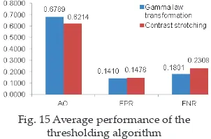
hyperintense lesion which is failed to detect by histogram. Therefore, histogram thresholding provides low performance for tumour segmentation in DWI. The errors for under-segmentation (FNR) are bigger than over-segmentation (FPR) for all cases. The shaded areas show the best average performance. Fig. 15 shows average performance of lesion segmentation by using both Gamma-law transformation and contrast stretching algorithm.

g. 15 Average performance of the thresholding algorithm

Fig. 15 Average performance of the thresholding algorithm

Gamma-law transformation algorithm provides higher AO which means beter similarity to the manual segmentation provided by neuroradiologists. For over-segmentation (FPR) and under-segmentation (FNR) evaluation, gamma-law transformation provides higher performance, while contrast stretching gives poorer result. Overall, gamma-law transformation algorithm provides beter segmentation results compared to contrast stretching.

B. gLCm

(11)

11

(a) Normal (b) Solid tumour

(c) Acute infarction

(d) Abscess (e)Haemorrhage (f) Acute infarction

(g) Acute Infarction

(h)Haemorrhage (f) Chronic infarction

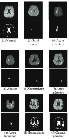
Fig. 16 Segmentation results. From top to bottom: (a) DWI for no patient and segmentation result of normal CSF, (b-g) SegmentatioFig. 16 Segmentation results. From top to

botom: (a) DWI for normal patient and

segmentation result of normal CSF, (b-g) Segmentation of hyperintense lesions, (h-f)

Segmentation of hypointense lesions For normal patient in Fig. 16(a), the DWI is separated into two parts which are brain tissue and CSF in the middle of the brain. The results show that the normal brain tissue is well separated from the CSF. No hyperintense lesion is detected. Fig. 16 (b-g) shows several hyperintense lesions and their segmentation results. As seen in the igures, the lesions are well segmented using the approach method. Similar evaluation is made for the hypointense lesions in Fig. 16 (h-f). Since the hypointense lesions and CSF share similar characteristics, hence both regions fall under the hypointense regions. Normal CSF can be characterized by looking at the symmetrical shape in the middle of the brain while for hypointense lesion, the shape is irregular.

C. segmentation performance Comparison

Fig. 17 shows average performance of lesion segmentation by using both GLCM

and thresholding. As discussed in the chapter VII, low MA, MAPE and rerr show low error, i.e high similarity with respect to the expert judgment. GLCM provides lower MA, MAPE and rerr compared to thresholding technique, which means more accurate. Overall, GLCM provides beter segmentation results compared to thresholding technique.

Fig. 17 Performance comparison between GLCM and thresholding

Fig. 17 Performance comparison between GLCM and thresholding

ix. ConCLusions

(12)

12

GLCM regions that were according to hyperintense and hypointense lesions were segmented. The result shows that the proposed methods can successfully segment the lesions and is suitable for analysis of DWI and for classiication purpose. Overall, GLCM provides beter segmentation accuracy compared to thresholding technique.

aCKnowLeDgment

The authors would like to thank Universiti Teknologi Malaysia (UTM) and Universiti Kebangsaan Malaysia Medical Centre (UKMMC) for collaboration in this research.

referenCes

[1] Malaysian Cancer Statistics – Data and Figure Peninsular Malaysia 2006, National Cancer Registry, Ministry of Health, Malaysia.

[2] American Cancer Society: Cancer Facts and Figures 2009. Atlanta, Ga: American Cancer Society, 2009.

[3] MAGNETOM Maestro Class: Difusion Weighted MRI of the Brain. From

brochure Siemens Medical Solutions that help.

[4] M. Ibrahim, N. John, M. Kabuka, A. Younis, “Hidden Markov models-based 3D MRI brain segmentation”, Elsevier Journal of Image and Vision Computing Vol.24, 2006, pp. 1065– 1079.

[5] S. J. Holdsworth, R. Bammer, “Magnetic Resonance Imaging Techniques:

fMRI, DWI, and PWI”, Seminars in

Neurology, 2008 Vol.28, No. 4.

[6] P. W. Schaefer, P. E. Grant, R. G. Gonzalez, “State of the Art:

Difusion-weighted MR imaging of the brain”, Annual Meetings of the Radiological Society of North America (RSNA), 2000, pp.331–345.

[7] S. K. Mukherji, T. L. Chenevert, M.

Castillo, “State of the Art:

Difusion-Weighted Magnetic Resonance

Imaging”, Journal of

Neuro-Ophthalmology Vol.22, No.2, 2002, pp. 118-122.

[8] R. Cardenes, R. de Luis-Garcia, M. Bach-Cuadra, “A multidimensional segmentation evaluation for medical image data” J. Computer Methods and Programs in Medicine, vol.96, 2009, pp.108-124.

[9] M.M. Trivedi, C.A. Harlow, R.W.

Conners, S. Goh, “Object detection based on gray level cooccurrence.” Computer Vision, Graphics, and Image Processing, 2:199-219, 1984.

[10] M.S. Khalil, D. Muhammad, M.K. Khan, Q. Al-Nuzaili, “Fingerprint

Veriication using Fingerprint

Texture.” Proceedings of the IEEE 2nd

International Conference on Machine Vision, pp. 27-31, 2009.

[11] M.M. Mokji, S.A.R. Abu Bakar, “Adaptive thresholding based on co-occurrence matrix edge information.” Proceedings of the 1st_{Asia International}

Conference on Modelling and Simulation, 2007.

[12] J. Webster (ed.), “Image Texture.” Wiley Encyclopedia of Electrical and Electronics Engineering, John Wiley &

Sons, Inc., 1999.

[13] N. Agani, S.A.R. Abu Bakar, S.H. Sheikh Salleh, “Application of texture analysis in echocardiography images for myocardial infarction tissue.” Jurnal Teknologi, pp.61-76, Jun 2007. [14] D.M-Ghoneim, “Cooccurrence

histogram for characterizing brain magnetic resonance images.” IEEE International Symposium on Signal Processing and Information Technology, 2009.

[15] H. S. Zadeh, F.R. Rad, et.al., “Comparison of multiwavelet, wavelet, Haralick, and shape features

for microcalcifcation classiication in

mammograms.” Elsevier Journals of

Patern Recognition, Vol.37, pp. 1973 –

1986, 2004.

(13)

13 [17] Haralick, R.M., Shanmugam, K.,

Dinstein, I., “Texture parameters for

image classiication.” IEEE Trans

Systems, Man, Cybernetics, 3: 610-621, 1973.

[18] M. Barnathan, J. Zhang, E. Miranda, et.al., “A Texture-Based Methodology for Identifying Tissue Type in Magnetic Resonance Images.” IEEE International Symposium on Biomedical Imaging (ISBI): From Nano to Macro, pp.464-467, 2008.

[19] M. Torabi, R.D. Ardekani, E. Fatemizadeh, “Discrimination between Alzheimer’s Disease and Control Group in MR-Images Based

on Texture Analysis Using Artiicial

Neural Network.” IEEE International Conference on Biomedical and Pharmaceutical Engineering, 2006.

[20] L.Wang, L. Tong, X. Liu, X. Li, C. Yu,

“Study on normal appearing white

mater of multiple sclerosis by texture

analysis and modelling with MRI.” IEEE International Conference on Information Acquisition, 2005.

[21] M. Ghazel, A. Traboulsee, R.K. Ward,

“Semi-Automated Segmentation of Multiple Sclerosis Lesions in Brain MRI using Texture Analysis.” IEEE International Symposium on Signal Processing and Information Technology, pp.6-10, 2006.

[22] J. Zhang, L. Wang, L. Tong, “Feature reduction and texture classiication

in MRI texture analysis of multiple sclerosis.” IEEE/ICME International Conference on Complex Medical Engineering, pp. 752-757, 2007.

[23] W. Lin, X. Zhou, G. Jing, “Texture

Analysis of MRI in Patients with Multiple Sclerosis Based on the

Gray-level Diference Statistics.” 1st

International Workshop on Education

Technology and Computer Science, pp.771-774, 2009.

[24] C. Chevreils, F. Cheriet, C´ Eric

Aubin, G. Grimard, “Texture Analysis for Automatic Segmentation of Intervertebral Disks of Scoliotic Spines from MR Images.” IEEE Transaction on Information Technology and Biomedicine, vol. 13, No. 4, pp. 608-620, 2009.

[25] S. Cha “Review Article: Update on Brain Tumor Imaging: From Anatomy to Physiology”, Journal of Neuroradiology, vol.27, pp.475-487, 2006.

[26] M.D.Hammer, L.R.Wechsler,

“Neuroimaging in ischemia and infarction.” Seminars in Neurology Vol.28, No. 4, 2008.

[27] R.T.Ullrich, L.W.Kracht, A.H.Jacobs

“Neuroimaging in patients with gliomas.” Seminars in Neurology, Vol.28, No. 4, 2008.

[28] O. Kastrup, I. Wanke, M. Maschke

(2008) Neuroimaging of infections of the central nervous system, Seminars in Neurology, Vol.28, No. 4, 2008. [29] J.F. Haddon, J.F. Boyce, “Co-occurrence

matrices for image analysis.” Electronics and Telecommunications Engineering Journal, pp.71-83, 1993. [30] N. Mohd Saad, S. A. R. Abu-Bakar,

Sobri Muda, Musa Mokji, “Automated Segmentation of Brain Lesion based on

Difusion-Weighted MRI using a Split

and Merge Approach”, Proceedings of 2010 IEEE-EMBS Conference on Biomedical Engineering & Sciences, IECBES 2010, 30th_{– 2}nd_{Dec. 2010, Kuala}

Lumpur, Malaysia.

[31] R.C. Gonzalez, R.E. Woods, Digital

Image Processing second edition, Prentice Hall, 2001.

[32] N. Mohd Saad, S. A. R. Abu-Bakar, Sobri Muda, M. M. Mokji, A. R. Abdullah, S. A. Mohd Chaculli, “Detection of

Brain Lesions in Difusion-weighted

Magnetic Resonance Images using Gray Level Co-occurrence Matrix”,

Proceedings of the World Engineering Congress 2010 (WEC 2010), Kuching,

Sarawak, Malaysia, pp.611-618. [33] Rosniza Roslan, Nursuriati Jamil, Rozi

Mahmud, “Skull Stripping of MRI Brain Images using Mathematical Morphology”, Proceedings of 2010 IEEE-EMBS Conference on Biomedical Engineering & Sciences (IECBES 2010), 30th_{– 2}nd_{Dec. 2010, Kuala Lumpur,}

(14)