Model-Driven Component Generation for Families of
Completeness Measures
Nurul Akmar Emran
School of Computer ScienceUniversity of Manchester Oxford Rd,Manchester,UK
[email protected]
Suzanne Embury
School of Computer ScienceUniversity of Manchester Oxford Rd,Manchester,UK
[email protected]
Paolo Missier
School of Computer ScienceUniversity of Manchester Oxford Rd,Manchester,UK
[email protected]
ABSTRACT
Completeness is a well-understood dimension of data qual-ity. In particular, measures of coverage can be used to assess the completeness of a data source, relative to someuniverse, for instance a collection of reference databases. We ob-serve that this definition is inherently and implicitly multi-dimensional: in principle, one can compute measures of cov-erage that are expressed as a combination of subset of the attributes in the data source schema. This generalization can be useful in several application domains, notably in the life sciences. This leads to the idea of domain-specific fam-ilies of completeness measures that users can choose from. Furthermore, individuals in the family can be specified as OLAP-type queries on a dimensional schema. In this paper we describe an initial data architecture to support and vali-date the idea, and show how dimensional completeness mea-sures can be supported in practice by extending the Quality View model [11].
1.
INTRODUCTION
Of the various forms of information quality (IQ) identi-fied in the literature, completeness has been one of the best studied and one of the most precisely defined. In particu-lar, it has been recognised that completeness is a complex quality, and that many different forms can be envisaged. A common distinction, for example, is to separate complete-ness of a data set in terms of the number of individuals represented (relative to the “true” population modelled by the data) from completeness in terms of the amount of data recorded about each individual (relative to the full amount of information that could possibly be collected about the in-dividual). These forms of completeness are commonly called coverageanddensity(after Naumannet al. [15]), and each demands a quite different approach to measurement.
We have been undertaking a study of the requirements for measuring IQ in various e-Science domains, with the aim of identifying patterns of IQ measure that are widely applica-ble, but which can be tailored for use in specific applications [11]. Recently, we have turned our attention to the issue of information completeness, which is of particular importance in many e-Science applications. A typical format forin sil-icoexperiments in e-Science is first to identify one or more public repositories which can provide the input to the ex-periment, to select from and clean up the data they provide, and then to execute the experiment (perhaps described in the form of a workflow [8]) over the selected data sets. As we shall show later in this paper, the completeness of the data
sets over which the experiment is run can have a significant effect on the correctness or usefulness of the results.
In order to elicit more precise requirements for complete-ness measurement in e-Science, we have looked specifically at the domain of SNP databases. A SNP (pronouncedsnip) is a single nucleotide polymorphism; that is, a change in a single base of a gene that is observed in a sufficiently large proportion of the population of a species to represent a specific trait within that population (rather than just a random mutation). Taken en masse, SNPs represent the genetic diversity of a species, and so are vital in helping to map phenotypic differences (such as susceptibility or re-sistance to specific diseases) to their corresponding genetic differences. Because of this, SNPs are typically used in com-parative studies of large sections of a species’ genome, and as such are particularly sensitive to completeness issues in the underlying data sets.
Our work has revealed a surprising diversity in complete-ness requirements, even within the standard coverage/density classifications found in the literature. Rather than one generic completeness measure, relative to the main population being accessed in an application, SNP scientists instead are con-cerned with the completeness of the data relative to certain specific dimensions. For example, for some kinds of SNP study, it is important that SNP for a specific set of strains of interest are included in the underlying data sets. For other applications, strains are not relevant; instead, coverage of certain regions of certain chromosomes is more important. Overall, we have identified a total of 20 dimensions in SNP data that might be important in assessing the completeness of SNP data sets for various applications.
Each such dimension represents a specific completeness measure, for which a “universe” of values must be compu-tationally accessible. Similarly, each combination of dimen-sions represents a completeness measure that may be of in-terest to some scientist. In other words, within a domain, there exists not one completeness measure, but a whole fam-ily of measures, defined by the dimensions of importance within the domain. Given this diversity, the following ques-tions arise:
• How can a specific completeness measure, i.e. a spe-cific member of the completeness family for the do-main, be rapidly and conveniently specified to support a particular application?
In this paper, we report on the results of our initial explo-rations of these questions. We first assess the literature on information completeness and draw from this previous work some general characteristics of completeness measures (Sec-tion 2). We then examine the specific completeness require-ments found in the SNP domain, and motivate the concept of dimensional completeness families proposed in this paper (Section 3). From this, we propose a model for dimensional completeness families (Section 4) and consider the software infrastructure that is needed to support completeness fam-ilies expressed in this model and how far it can be auto-matically generated from the model (Section 5). Finally, we conclude (Section 6).
2.
MEASURES OF COMPLETENESS
Completeness of information is included as a key dimen-sion of IQ in all the major taxonomies proposed in the lit-erature (e.g. [1, 3, 17, 22]). Unlike many other measures, completeness is conceptually very simple: completeness is typically defined as the ratio of the size of the data set of interest relative to the size of the “complete” data set. This “complete” data set (which, in this paper, we term the uni-verse) may refer to the state of the real world (e.g. the number of genes actually present in the human genome) or to some stored data set that is believed to be a good ap-proximation of the real world (e.g. the GenBank database1
, which records details of the majority of well-established, ex-perimentally determined human genes, i.e., the set of known genes). Completeness measures using the former kind of universe are sometimes referred to asabsolute completeness measures (with a similar concept found in the literature as the completeness approximation against a reference relation [20]), while the latter are referred to asrelative completeness. In specifying a particular completeness measure, there-fore, our two main tasks are to define how we measure the size of a data set, and to identify the contents or character-istics of the universe against which completeness should be assessed. Note that the size measure must be applicable to both the data set under study, and to the universe, in order to produce a meaningful ratio of the two quantities (or else two separate but comparable measures must be defined).
Two main approaches to measuring the size of a data set can be seen in the literature: counting the number of individ-uals (given the namecoverageby Naumannet al. [15]) and assessing the amount of information available about each recorded individual (given the namedensityby Naumannet al. [15]). Both are useful in some situations, and less useful in others. And both bring their own specific challenges in terms of forming precise and automatable quality measures. For example, obtaining an accurate count of the number of individuals recorded in a data set is complicated by the need to deal with duplicates, while assessing the amount of information recorded about one individual is complicated by issues regarding precision of different data representations.
Ballou and Pazer, for example, discuss the difficulties of assessing the relative information content of the temperature values “below freezing” and “20F” [2]. Clearly the former is less complete than the latter, but how is this difference to be measured precisely? Because of this difficulty, current density measures distinguish only between null and non-null values in terms of information content. For example,
Scan-1
http://www.ncbi.nlm.nih.gov/Genbank/GenbankOverview.html
napieco and Batini proposed a hierarchy of density mea-sures based upon counting the non-null values in data sets at the level of a tuple, a column or a complete relations [20]. Similar measures were also defined by Naumannet al. [15], Martinez and Hammer [10] and Motro and Rakov [14]. Such measures are meaningful in contexts where null has a clear and unambiguous meaning - such as in integrated data sets where null values have been inserted whenever the underly-ing data sources did not contain the information needed to fully populate the attributes of the integrated data. They are less useful in contexts where null has other meanings beyond (and including) “unknown”. For example, in many relational data models, null is also used to indicate that a value is inapplicable or empty, as well as when its value is unknown. In such cases, a plain count of nulls will not give a reliable indication of the data completeness.
Even aside from the issue of deduplication/object iden-tity, the specification of universes for completeness measures is a challenging task. Ideally, of course, we would assess completeness against the state of the real world, but this is either impractical or impossible in the vast majority of cases. It is necessary, therefore, to define some proxy for the state of the real world that exists in the technical world and that is sufficiently representative of the real world state to allow meaningful completeness assessments to be made. Two main approaches to universe specification can be dis-tinguished in the literature: virtual (or intensional) and ma-terialised (or extensional).
Virtual universe specifications are defined using rules that describe the relevant characteristics of the complete data set without enumerating it in full. These specifications may be stated explicitly, as part of the measure, or may be implic-itly assumed. For example, forms of density measures that are based on counting nulls, such as that of Scannapieco and Batini described above [20], are based on an implicit virtual specification of the universe. In these measures, the universe is assumed to have the same number of individuals and attributes as in the data set being measured, but with the additional knowledge that each attribute is also non-null. Although this specification of the universe does not tell us exactly what values are held by each tuple attribute, it gives enough information for us to be able to assess the number of missing values.
An example of an explicit virtual universe specification, this time in terms of a coverage measure, was given in an early paper on completeness by Motro [13]. In this work, Motro proposed that the data administrator for a data set could give rules describing the set of individuals in the real world data. An example based on the flight information do-main used by Motro is the statement that there is one flight daily between Los Angeles and New York. A database of flights can be checked for completeness relative to this por-tion of the real world, even though the exact set of flights actually scheduled by this airline is unknown. Another ex-ample of this kind of universe specification is given by Ba-tini and Scannapieco in the context of public administra-tion databases [3]. If the approximate populaadministra-tion of a city is known, then the completeness of a database of residents of that city can be estimated based on this value alone.
ob-vious of these is the problem of false positives in the data set, which cannot always be detected by these measures and which can therefore distort the completeness results. For example, the residents database just mentioned might also contain the names of many people who no longer live in the city, and who are not included in the population esti-mate. The virtual universe specification does not allow us to rule such residents out of the calculation. A further issue is that of maintenance of the rules defining the universe. If these rules do not accurately describe the real world (either because of a change in the world or because they were incor-rectly specified) then the completeness measures that result will be of doubtful value.
It is also the case that many (most?) universes cannot be specified in this intensional manner, either because of the complexity of their semantics or because they contain data describing collections of natural kinds that cannot be encap-sulated by neat rules. The only way to describe the set of genes in the human genome (whether actual or as currently known), for example, is to list them in terms of the artifi-cial names given to them by scientists. For these kinds of domains, it is necessary to define the universe extensionally, by enumerating its members.
In cases where a single database or resource exists that is a close approximation of the real world, then this can be used as a proxy universe and completeness of other data sets can be measured against it [20]. For example, for prac-tical purposes, the GenBank database referred to earlier is a good proxy universe for the set of known genes (and even for the set of genes that actually exist, given the extreme difficulty of obtaining this information). Completeness of any database of genes can be reliably assessed against its contents.
The number of domains where a reliable single reference resource for completeness exists are small, however. An al-ternative approach is to construct a universe from the total amount of information that is known; i.e., to construct a sin-gle reference set by integrating the multiple sources that are available. Naumannet al.made use of this idea in their pro-posal for a coverage measure based on the idea of auniversal relation[15]. Assuming a LAV integration approach, these authors define the universal relation to be a single relation containing the outer join of all the views exported by the individual sources2
. This universal relation is then used to assess the completeness of the individual sources, by deter-mining what proportion of the tuples in the full universal re-lation are supplied by the source being assessed. A universe of this kind will give accurate completeness values in situa-tions where the underlying sources by and large represent a horizontal decomposition of the data being integrated (i.e., where there is an approximate one-to-one correspondence between tuples in the universal relation and individuals in the real world set). In other cases, where (for example) the underlying source views represent a vertical or mixed de-composition of the real world information, the number of tuples in the universal relation will be artificially inflated and its tuples may not correspond to meaningful real world entities. This would occur, for example, whenever foreign
2
Naumannet al. define a special form of join operator for this purpose that not only fills in with nulls when values are missing in a source relation, but also merges values when two or more joined views provide a value for a given attribute [15].
keys within the views represent one-to-many relationships of high cardinality. In such cases, some other form of uni-verse specification must be found.
One advantage of materialised universes is that they have the potential to handle false positives correctly, so that they do not distort the completeness measure. However, this is only the case when the data set under study is not part of the set from which the universe is computed are under study. A key (though often unstated) assumption behind this “inte-gration” approach to universe formation is that the sources that make up the universe are accurate (that is, they do not themselves contain false positives). In some domains, it may be easier to manually create and maintain a single reference source for completeness measurement, rather than attempt-ing to guarantee the accuracy of all the sources from which the universe might otherwise be automatically constructed. Having examined the arsenal of completeness measures proposed to date within the literature, in the next section we will consider how well the measures match up to the requirements for completeness assessment with an example e-Science domain.
3.
COMPLETENESS IN SNP DATABASES:
A MOTIVATING EXAMPLE
3.1
Overview
One of the primary concerns of biologists is to increase our understanding of the relationship between the genes that an organism acquires from its parents (i.e., its genotype), and the structural and behavioural characteristics it will display as a result (i.e., its phenotype). For example, eye colour in humans (phenotype) is known to be governed by a group of genes, including EYCL1, EYCL2 and EYCL3. Discovering such relationships is challenging, especially for phenotypic traits that are qualitative rather that quantitative, such as those governing susceptibility or resistance to various dis-eases, and which are governed by a complex interplay of many genes spread across disparate locations in the organ-ism’s full genetic sequence.
Single nucleotide polymorphisms (SNPs for short, pro-nounced “snips”) are a specific type of genetic variation that can be used to support many forms of analysis aimed at generating or testing hypotheses relating to such relation-ships. A SNP is a variation in a single nucleotide base (and therefore in a single gene) that is seen in at least 1% of the population of the species under study [5]. SNPs are signifi-cant because they can highlight potential candidate genes for specific phenotypic behaviours, through comparative stud-ies. The underlying assumption behind many SNP studies is that the genetic factors (i.e., variation) that contribute to an increased risk for a particular condition or disease should be detected at higher rates in the population which exhibits the condition compared to the population which does not [5]. To give a small and unrealistic example of this, suppose one mouse strain is likely to develop a particular congeni-tal defect while another strain is not. If gene A1 has the sequence “AAAAA” in the first strain, but the sequence “AACAA” in the second, then the presence of the SNP at the third allele 3
may indicate that the gene has a role in
3
Figure 1: Completeness differences in three human SNP databases involving 74 genes.
(taken from [9])
the development processes that lead to the defect.
SNP data has so far proven to be of value in three main types of genomics analysis, namely, association studies, gene mapping and evolutionary biology studies [6, 19, 21]. In association studies, for example, SNPs have been used to identify genetic factors correlated with complex diseases [5, 7, 24]. Because of this, efforts to discover and document new SNPs have gained momentum in recent years [5, 23], result-ing in the establishment of a number of public and private databases [5, 23]. For example, in April 1999, a total of 7000 SNPs had been deposited into the major public databases [5], while by January 2002 some 4 million SNPs had been deposited in the dbSNP database alone [9]. Since then, many other public databases and repositories have been es-tablished, including databases like Perlegen4
, GeneSNP5
, PharmGKB6
and HOWDY7
[9].
The vast amount of SNP data now available holds out the possibility for supporting many forms of genomic analysis. However, there is a growing concern with the SNP user com-munity regarding the quality of data in these databases, and in particular regarding sharp variations in quality from one database to the next [5, 9, 18]. Although there are some concerns about false positive rates [4], for many scientists, the more immediate concern regards the completeness of the SNP data sets chosen as the foundation for their analyses. For example, Marshet al. undertook a study of three well-known human SNP databases for 74 human genes: CGAP-GAI8
, LEELAB9
and HOWDY [9]. Their work revealed a significant lack of overlap between the databases, as shown by the Venn diagram in Figure 1. As a result, they cautioned against performing analyses over only a single database (or a small selection) because this would result in incomplete sets of genetic variants being uncovered.
Given this diversity, and the lack of a single reliable ref-erence source for SNPs, a coverage measure such as that
4
Perlegen - http://www.perlegen.com
5
GeneSNP - http://www.genome.utah.edu/genesnps/
6
PharmGKB - http://pharmgkb.org
7
HOWDY - http://howdy.jst.go.jp/HOWDY
8
CGAP-GAI - http://gai.nci.nih.gov/cgap-gai/
9
LEELAB - http://www.bioinformatics.ucla.edu/snp/
Figure 2: SNP coverage in the Perlegen data set.
(Taken from [12])
Figure 3: SNP coverage in Ensembl data set.
(Taken from [12])
proposed by Naumann et al. [15] would seem to be ap-propriate. SNP databases tend to contain only SNP records (i.e., they contain horizontal fragmentations of the complete set of SNPs) plus associated metadata, so the universal rela-tion formed by their integrarela-tion would correspond roughly to the total number of known SNPs. However, complete-ness relative to the total number of known SNPs is rarely useful in SNP analyses, which tend to be focussed on spe-cific scenarios and spespe-cific hypotheses, and which are thus concerned with completeness of their data relative to a sub-set of the available SNP data, rather than the global SNP universe. For instance, SNP studies are typically concerned with a specific set of strains or a specific species, and with a particular region of a particular chromosome thought to be the location of the genes of relevance. An individual sci-entist, therefore, will be concerned over time not with one standard form of completeness, but with a whole variety of completess forms, each tailored to the needs of the specific analysis in hand.
exam-ination. Even if a more general form of SNP completeness measure had been available to Petko and the team, it would have been of little value unless it could have assessed the specific completeness of data sets relative to these partic-ular criteria (strain, species and QTL). As it was, without any way to assess the validity of their specific assumptions about the completeness of the data sets used in the study, the confidence in the results must be reduced [16].
A more recent study of SNP database completeness dis-covered that sources can vary widely in the forms of coverage they achieve, as well as in degree of overall coverage. Fig-ures 2 and 3 show the coverage of SNP data in two well known sources for Mouse SNPs: Perlegen and Ensembl10
. The Perlegen data set resulted from a systematic effort to provide complete coverage across the genome for fifteen se-lected mouse strains; hence it has good positional coverage, but very poor coverage across the full set of strains (even if only mouse strains are considered). Ensembl, by contrast, is a general repository for SNPs of all kinds (as well as much other biological data). As the figure shows, it contains SNPs for a much wider range of strains than Perlegen, but with a much patchier coverage across the mouse genome.
3.2
The SNP Completeness Family
The principal lesson to be drawn from this examination of completeness requirements in an e-Science domain is that even within a single application area we can expect to see not one but many forms of completeness, whether density types measures or (as in this particular case) coverage-style measures. We can also see that certain attributes of the data sets under study make sense as the basis of complete-ness measures, while others do not. In order to discover the characteristics of an attribute that rule it into one category or the other, it is instructive to attempt to classify the in-formation commonly stored about SNPs according to their potential role in a completeness measure.
Some common SNP attributes are:
1. the unique identifier for the SNP,
2. the chromosome on which the SNP is located,
3. the base position on the chromosome at which the SNP is located (locus),
4. the allele determined for the SNP,
5. the submitter institution or lab which was responsible for experimentally determining the SNP,
6. the strains in which the SNP is known to occur,
7. the species of organism from which the evidence for the SNP was experimentally collected,
8. the “build” (i.e., version) of the species’ genome that was used to identify the SNP and in terms of which its position is specified, and
9. the sources where SNPs have been deposited.
Some of these are good candidates for completeness mea-sures. We have already talked about completeness relative to a set of strains of interest (or the full set of strains for an organism), and about completeness of SNP coverage across
10
Ensembl - http://www.ensembl.org/index.html
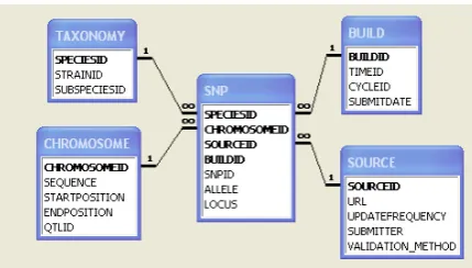
Figure 4: SNP Schema.
a chromosome or genome. It might also be reasonable in cer-tain circumstances to ask for a SNP data set that includes all the data submitted by a particular lab (for example, if the lab is known to have undertaken a thorough study of certain QTLs relevant to a particular disease). It seems less sensible to ask for a data set that is complete relative to all possible alleles. There are only a small number of nu-cleotide bases that occur in DNA (an example, incidentally, of a universe that is very conveniently defined virtually, as a set of letters) and it does not seem likely that a data set which contains an example of a SNP for each of them would have any useful biological or statistical properties. Obvi-ously, the unique identifier for a SNP is going to make a very uninteresting set of SNPs by itself.
If we construct a model of SNP data based around these attributes, it would look something like the schema shown in Figure 4. Readers may notice the similarity of this schema to the star schema form commonly used in data warehouses. If we look further at this model, we see that the attributes around which completeness measures can be envisaged ap-pear in the model as dimensions, while the attributes which are not useful in this way appear on the central fact ta-ble. In other words, the completeness attributes refer to a set of values that exists in some sense independently of the SNP data, but which describes its context or meaning (as a kind of metadata). For example, the set of strains is defined independently of the SNP data, but selected strains are as-sociated with specific SNPs in order to describe the context in which the SNP was observed.
What we observe, therefore, is that SNP data is multi-dimensional (including some hierarchical dimensions: a SNP at a particular position is a member of one or more QTLs, which are in turn components of chromosomes, which them-selves combine to form a species’ genotype). Each such di-mension is associated with its own universe. However, the dimension is not measured for completeness by itself. In-stead, we measure coverage of the dimension within the data set being measured, a data set in which the main data type is the fact data, not the dimension. For different applications (e.g., different analysis types), different completeness dimen-sions will be important to differing degrees and in different combinations. Therefore, the dimensional model actually defines a whole family of possible completeness measures, which the user should be able to select from as each new analysis type is encountered.
provided a dimensional model can be created. For example, if we consider a database of clinical patient observations, we might wish to assess its completeness relative to the time at which the observations took place (when studying effects on patients of a time when mRSA was known to be present in certain institutions), to the hospitals at which the obser-vations were made (when wishing to distinguish good and bad practice at institutions), to the demographics of the patients who are the subject of the observations (when at-tempting to study the course of a disease amongst certain income/occupation groups). Similarly, sales data might be assessed for completeness relative to spatial criteria based on the location of the sale or the type of goods sold.
On the assumption that these multi-dimensional complete-ness families are of wider applicability than just SNP data, a number of questions arise:
• How can such families of completeness measures be specified?
• How can a user of the family specify that a particu-lar measure (i.e. a member of the family) should be invoked in a specific situation?
• What software infrastructure is needed to support the efficient measurement of completeness relative to any of the specific measures that belong to a family?
In the next section, we describe the results of our initial investigations into these questions.
4.
MULTI-DIMENSIONAL COMPLETENESS
FAMILIES
As we have said, to define a completeness measure for data setsDS, it is necessary to define both the universe of values Uand a means of assessing the size of bothU andDS. Since our completeness measure families are multi-dimensional, we must also define the set of dimensions that provide the skele-ton for the family, and some means by which the complete-ness scores for the individual dimensions can be aggregated together, to give a final value for the completeness of the data set as a whole. We will discuss each of these compo-nents in turn.
4.1
Dimension Specification
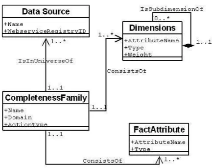
The most essential part of the specification of a complete-ness family is a description of the type of data that will be assessed for completeness (the “fact” data) and the dimen-sions along which its completeness will be measured. The UML class diagram shown in Figure 5 outlines the informa-tion to be provided (along with some further components which will be described later in this section). We assume that there is just one “fact” data type, but that it may have multiple attributes. There may also be one or more dimension attributes, which may be grouped together into hierarchies.
As well as defining the individual measures within the family, the specification of the dimension and fact attributes also defines the schema which will be used to represent the data values during completeness assessment.
4.2
Universe Specification
For each dimension, we need information about the uni-verse of values that represent its complete extent. It may
Figure 5: A Completeness Family Model.
be possible in some cases that the universe for a dimension may be specified concisely either by intensional or exten-sional means. In general, however, we cannot rely on either of these possibilities. We therefore adapt the idea of uni-versal relations described earlier to our multi-dimensional setting. As with the proposal from Naumann et al. [15], we assume that the person specifying the completeness fam-ily is able to identify a collection of data sources that will together make up the universe for all dimensions for the do-main. An individual universe then consists of the union of all discrete values that appear in the dimensional attribute in all the data sources defined by the family designer.
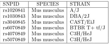
For example, consider the (unreasonably small) SNP data sources shown in Tables 1 and 2. If these two sources are specified as forming the basis of the universe for a SNP com-pleteness family, then the universe for thespeciesdimension will be:
{“Mus musculus”}
and the universe for thestraindomain will be:
{“A/J”,“129S1/SvImJ”,“BTBR T+ tf/J”, “DBA/2J”,“CAST/EiJ”,“C3H/HeJ”}
Since the format of the data sources specified as the universe for the family may vary dramatically, it is also necessary for the family designer to provide for each data source the URL of a Web service that will extract the sets of discrete values contained within it for each dimension attribute. The data should be provided in the format described by the dimen-sions and the fact table.
4.3
Dimensional Completeness
We adopt a simple ratio metric for the completeness mea-sures for individual dimensions. If the data set being as-sessed contains the setviof discrete values for dimensioni, then its completeness relative to the specified universe for that dimension,ui, is given by:
ci(ds) =|ui∩vi|/|ui|
SNPID SPECIES STRAIN rs2020841 Mus musculus A/J rs2030843 Mus musculus A/J rs2040845 Mus musculus A/J
rs2060840 Mus musculus 129S1/SvImJ rs2070849 Mus musculus BTBR T+ tf/J
Table 1: SNP Data Source 1.
SNPID SPECIES STRAIN
rs1020841 Mus musculus A/J rs1030843 Mus musculus DBA/2J rs3040845 Mus musculus CAST/EiJ rs6070849 Mus musculus BTBR T+ tf/J rs4070849 Mus musculus C3H/HeJ rs5070849 Mus musculus C3H/HeJ
Table 2: SNP Data Source 2.
4.4
Aggregating Dimensional Completeness
Since users of a family may be concerned with more than one completeness dimension at a time, we must have some way of aggregating the individual dimension scores just de-scribed into a single over-arching completeness score for the data set as a whole (relative to the dimensions of interest). In this first version of the family model, we adopt a simple weighted average approach, since this will preserve the ratio nature of the score as well as balancing the strengths and weaknesses of the selected dimensions against one another. Other approaches may well prove to be more appropriate after further work.
Rather than fixing the weightings, we allow designers of families to specify their preferred default weights for each dimension. As we shall later discuss, these weights can be over-ridden at run-time, when a specific completeness mea-sure from within the family is invoked.
4.5
Completeness Families in Use
Given the information just described, our goal is to (auto-matically, as far as possible) generate a software component or components that can implement the completeness fam-ily. We use as the basis for this generation the framework provided by the Qurator project11
. The Qurator framework supports model-driven generation of components for IQ as-sessment calledquality views[11]. A quality view or QV for short (illustrated in Figure 6) is a layered component that takes in a data set, classifies each element in the data set according to its quality according to some domain-specific measure, and outputs a version of the data set, transformed in some way according to the classification. For example, a very common transformation involves filtering out elements of the data set that do not meet some pre-defined quality standard. The QV also takes in some arbitrary parame-ters, and exports a report giving the quality classifications assigned to each item of the input data set.
As the figure shows, internally, quality views are layered components. The first layer consists of components that can gather evidence about the data elements that pertains to their quality. The middle layer takes this evidence as input, and applies a decision procedure that classifies each data set element in terms of its quality, as indicated by the evidence
11
www.qurator.org
Gather Evidence needed for Quality Assessment
Transform Input Elements Based on Quality Class/Score Classify/Score Input Elements According to their Quality
DS'
DS Auxiliary Parameters
Quality Report
Figure 6: The Qurator Quality View Pattern.
received. These quality classifications are then passed on to the third layer, the “action” layer, which transforms the input elements based on their quality.
QVs can be specified as a high-level model which is then compiled into a Web service that implements the black-box behaviour just described. These Web services can then be incorporated into the user’s preferred information manipu-lation environments, to make them “quality aware”. Ideally, we would like our completeness families to be manifested as QVs, so that they are easy to adopt for users already famil-iar with other forms of IQ measurement in QV form. Since we can pass arbitrary parameters to QVs, this is relatively easy to manage.
Completeness is an aggregate measure that can only be sensibly applied to sets of data, rather than to individual values. Therefore, the input data set for a completeness family QV (cfQV) must be a set of data sets, each of which is to be assessed for completeness. (Of course, the set can be a singleton set if only one data set is to be assessed for completeness.) In this first version of the cfQV model, we assume that the caller wishes to assess the completeness of one or more of the sources specified in the universe for the family, and therefore the input data set is simply a list of the identifying names given to the sources of interest when the family was defined. In future version of our work, we will expand on this initial simplistic definition.
The caller must also specify which dimensions are to be used for assessment of completeness, i.e., which of the collec-tion of completeness measures embodied by the family are to be invoked on this occasion. The dimensions are specified as a list of names in an arbitrary parameter to the QV. They can optionally be accompanied by weights for the dimen-sions if the caller does not wish to make use of the default weights defined for the family.
dimen-sions. The exact nature of this computation is described in Section 5. The middle layer applies the weighted average to the individual dimension completeness scores, and produces an overall completeness score. The action layer then per-forms whatever action has been specified by the designer of the family (see Figure 5), for example, as an XSLT rule set. The model shown in Figure 5 contains all the information needed to allow us to generate this form of QV automati-cally. However, a further important design choice has yet to be made, as we shall discuss in the next section.
5.
SOFTWARE INFRASTRUCTURE
The simplest implementation of the completeness family quality views just described is one in which all the informa-tion needed for completeness assessment is gathered from the universe of sources on demand, at the time when the cfQV is invoked for some specific measure. However, this is unlikely to be very efficient, especially if the number of sources in the universe is large, if the universes for any of the dimensions are large, or if the number of dimensions of interest to the caller are significantly less than the total num-ber available. If the cfQV is to be invoked regularly, then an alternative approach would be to materialise the various dimensional universes in central warehouse. Although the effort of constructing (and perhaps maintaining) this ware-house might be considerable, it could be worthwhile if a large number of users are accessing the family, each wishing to make use of a slightly different combination of dimensions and/or weights.
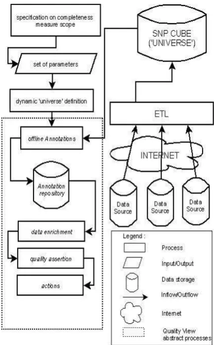
This would require some infrastructure beyond the bor-ders of the QV component, a departure from our earlier work on QVs. We therefore chose to explore this option, with the aim of determining the costs and potential benefits of the approach, and of discovering how much of the necessary soft-ware infrastructure could be automatically generated from the completeness family model. Figure 7 shows the full set of components. At the top left, we have the specification of the completeness family, in terms of the high-level model. This is used to create and configure the components needed for the rest of the infrastructure. On the right of the dia-gram is the infrastructure needed to create the warehouse of universe data needed to support the cfQV. We have already noted the similarity of our data representation (shown in Figure 4) to a star schema. Because of this, we chose to use data warehouse technology to implement the materialised universe view12
. This supports queries over a wide variety of combinations of dimensions and sources, so that the full range of completeness measures embodied by the family can be efficiently and seamlessly supported.
The warehouse is populated from the sources using the Clover ETL framework13
. Data is extracted from the sources using the specified web services, and is then transformed and loaded into the materialised universe source. At present, we have considered only the initial creation of this ware-house. In future, we will of course have to consider the infrastructure needed to maintain it when the underlying sources change. However, in essence, this is a very standard warehouse refresh process, and we should be able to make use of the wealth of expertise and tools available in this area.
12
MySQL (http://www.mysql.com) is used as the database management system.
13
Clover.ETL - http://cloveretl.berlios.de/
Figure 7: The cfQV Software Infrastructure.
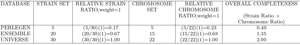
At the bottom left of the figure is the QV component that is created automatically from the cfQV model in order to act as the point of access to individual members of the complete-ness measure family. When this QV is invoked, the evidence gathering functions issue queries to the materialised universe in order to compute the completeness of the selected sources relative to the selected dimensions. For example, suppose that a cfQV has been defined for SNP data, with a variety of well known SNP sources as universes, and the dimensions shown in Figure 4. Suppose further that some user invokes the resulting cfQV requesting that completeness of the Per-legen and Ensembl data sources relative to the dimensions ofstrainandchromosome, with equal weights. The quality evidence function would begin by issuing the following query to warehouse that stores the family universes:
SELECT DISTINCT(t.strainid), DISTINCT(s.chromosomeid) FROM taxonomy t JOIN snp s ON t.speciesid = s.speciesid;
Then, to retrieve the set of values in the specific sources, it issues queries of the form:
FROM taxonomy t JOIN snp s ON t.speciesid = s.speciesid; WHERE s.sourceid = "perlegen";
The resulting ratios are passed on to the quality classifica-tion layer of the cfQV, which computes their average, and outputs the results in the quality report.
Table 3 shows an example of the SNP cfQV at work.
6.
CONCLUSION
The work presented in this paper stems from the obser-vation that, in several applications domains, the notion of data completeness can be expressed quite naturally in terms of multiple dimensions. In the context of SNP data analy-sis for biological applications, for example, we have been able to identify a number of dimensions (including chro-mosome, strain, and species) that scientists can use, either individually or in combination, to express useful measures of completeness. Our definition of dimensional completeness assumes that, for each dimension, completeness is measured with respect to a universe of values that is available for that dimension. This leads naturally to the idea of expressing complex completeness measures as OLAP-type queries on a dimensional schema.
The study presented in the paper is a preliminary investi-gation into this idea, and is limited to a few, simple example queries. Nevertheless, we have shown how dimensional com-pleteness measures can be supported in practice by leverag-ing our existleverag-ing Qurator framework [11], proposed in earlier work. In particular, we are implementing a first prototype to show how we can rank a collection of data sources (e.g., a collection of SNP databases) by extending the Quality View model that is at the core of Qurator. In the full implemen-tation, users will be able to specify the ranking criteria at run-time, as aggregation queries on the dimensional com-pleteness model.
7.
REFERENCES
[1] D. P. Ballou and H. L. Pazer. Modeling data and process quality in multi-input, multi-output information systems.Management Science, 31(2):150–162, 1985.
[2] D. P. Ballou and H. L. Pazer. Modeling completeness versus consistency tradeoffs in information decision contexts.IEEE Transactions On Knowledge and Data Engineering, 15:240–243, 2003.
[3] C. Batini and M. Scannapieco.Data Quality : concepts, methodologies and techniques. Springer, Berlin, 1998.
[4] A. Brass. Private communication, 2007. [5] A. J. Brookes. The essence of SNPs.Gene,
234:177–186, 1999.
[6] L. Comai and S. Henikoff. TILING: practical single-nucleotide mutation discovery.The Plant Journal, 45:684–694, 2006.
[7] E. Halperin, G. Kimmel, and R. Shamir. Tag SNP selection in genotype data for maximizing SNP prediction accuracy.Bioinformatics, 21:195–203, 2005. [8] B. Lud¨ascher, I. Altintas, C. Berkley, D. Higgins,
E. Jaeger, M. Jones, E. A. Lee, J. Tao, and Y. Zhao. Scientific workflow management and the Kepler system.Concurrency and Computation : Practice and Experience, 18:1039–1065, 2005.
[9] S. Marsh, P. Kwok, and L. H. Mcleod. SNP database and pharmacogenetics: Great start, but a long way to go.Human Mutation, 20:174–179, 2002.
[10] A. Martinez and J. Hammer. Making quality count in biological data sources. InIQIS, pages 16–27. ACM, 2005.
[11] P. Missier, S. Embury, R. Greenwood, A. Preece, and B. Jin. Quality views: capturing and exploiting the user perspective on data quality. InProceedings of the 32nd international conference on VLDB ’06, pages 977–988. ACM Press, 2006.
[12] P. Missier, S. Embury, C. Hedeler, M. Greenwood, J. Pennock, and A. Brass. Accelerating disease gene identification through integrated SNP data analysis. InProceedings 4th International Workshop on Data Integration in the Life Sciences, pages 215–230. Springer, 2007.
[13] A. Motro. Integrity = validity + completeness.ACM Transactions on Database Systems, 14(4):480–502, 1989.
[14] A. Motro and I. Rakov. Estimating the quality of databases. InProceedings of the Third International Conference on Flexible Query Answering Systems, pages 298–307. Springer-Verlag, 1998.
[15] F. Naumann, J. Freytag, and U. Leser. Completeness of integrated information sources.Information Systems, 29(7):583–615, 2004.
[16] P. M. Petkov, Y. Ding, M. A. Cassell, W. Zhang, G. Wagner, E. E. Sargent, S. Asquith, V. Crew, K. A.Johnson, phil Robinson, V. E. Scott, and M. V. Wiles. An efficient SNP system for mouse genome scanning and elucidating strain relationship.Genome Research, 14:1806–1811, 2004.
[17] T. Redman.Data Quality for the Information Age. Artech House, Boston, MA, 1996.
[18] D. E. Reich, S. B. Gabriel, and D. Atshuler. Quality and completeness of SNP databases.Nature Genetics, 33(Brief Communication):457–458, 2003.
[19] D. Savage, J. Batley, T. Erwin, E. Logan, C. G. Love, G. A. Lim, E. Mongin, G. Barker, G. C. Spangenberg, and D. Edwards. SNPServer: a real-time SNP discovery tool.Nucleic Acids Research, 33(Web Server Issue):493–495, 2005.
[20] M. Scannapieco and C. Batini. Completeness in the relational model: a comprehensive framework. InMIT Conference on Information Quality (IQ), pages 333–345, 2004.
[21] S. Sherry, M. Ward, J. Baker, E. Phan, E. Smigielski, and K. Sirotkin. dbSNP: the ncbi database of genetic variation.Nucleic Acids Research, 29:308–311, 2001. [22] R. Wang and D. Strong. Beyond accuracy: what data
quality means to data consumers.Journal of Management Information Systems, 12(4):5–33, 1996. [23] H. Xu, S. G. Gregory, E. R. Hauser, J. E. Stenger,
M. A. P. Vance, J. M. Vance, S. Zuchner, and M. A. Hause. SNPselector: a web tool from selecting SNPs for genetic association studies.Bioinformatics, 21(22):4181–4186, 2005.
DATABASE STRAIN SET RELATIVE STRAIN CHROMOSOME RELATIVE OVERALL COMPLETENESS
RATIO,weight=1 SET CHROMOSOME
RATIO,weight=1 (Strain Ratio + Chromosome Ratio)
PERLEGEN 5 (5/30)(1)=0.17 5 (5/22)(1)=0.23 0.40
ENSEMBLE 20 (20/30)(1)=0.67 15 (15/22)(1)=0.68 1.35
UNIVERSE 30 (30/30)(1)=1.00 22 (22/22)(1)=1.00 2.00
![Figure 1: Completeness differences in three humanSNP databases involving 74 genes.(taken from [9])](https://thumb-ap.123doks.com/thumbv2/123dok/663556.81414/4.595.94.254.56.208/figure-completeness-dierences-humansnp-databases-involving-genes-taken.webp)