DOI: 10.12928/TELKOMNIKA.v13i3.1805 976
RVM Classification of Hyperspectral Images Based on
Wavelet Kernel Non-negative Matrix Fractorization
Lin Bai1, Defa Hu*2, Meng Hui3, Yanbo Li4
1,3,4
School of Electronics and Control Engineering, Chang'An University, Xi’An 710064, Shaanxi, China
2
School of Computer and Information Engineering, Hunan University of Commerce, Changsha 410205, Hunan, China
*Corresponding author, e-mail: [email protected]
Abstract
A novel kernel framework for hyperspectral image classification based on relevance vector machine (RVM) is presented in this paper. The new feature extraction algorithm based on Mexican hat wavelet kernel non-negative matrix factorization (WKNMF) for hyperspectral remote sensing images is proposed. By using the feature of multi-resolution analysis, the new method of nonlinear mapping capability based on kernel NMF can be improved. The new classification framework of hyperspectral image data combined with the novel WKNMF and RVM. The simulation experimental results on HYDICE and AVIRIS data sets are both show that the classification accuracy of proposed method compared with other experiment methods even can be improved over 10% in some cases and the classification precision of small sample data area can be improved effectively.
Keywords: hyperspectral classification, non-negative matrix factorization, relevance vector machine, kernel method
Copyright © 2015 Universitas Ahmad Dahlan. All rights reserved.
1. Introduction
It is well know that each material has its own specific electromagnetic radiation spectrum characteristic. Using hyperspectral imagery (HSI) sensors, it is possible to recognize materials and their physical states by measuring the spectrum of the electromagnetic energy they reflect or emit. The spectral data which consist of hundreds of bands are usually acquired by a remote platform, such as a satellite or an aircraft, and all bands are available at increasing spatial and spectral resolutions. After 30 years of development, HSI technology has not only been widely used in military, but also has been successfully applied in ocean remote sensing, vegetation surveys, geological mapping, environmental monitoring and other civilian areas [1, 2].
Due to the state of art of sensor technology developed recently, an increasing number of spectral bands have become available. Huge volumes of remote sensing images are continuously being acquired and archived. This tremendous amount of high spectral resolution imagery has dramatically increased the information source and increased the volume of imagery stored [2, 3].
However, the excessive HSI data increase the difficulty of image processing and analysis. Such as supervised classification of HSI images is a very challenging task due to the generally unfavorable ratio between the large number of spectral bands and the limited number of training samples available a priori, which results in the ‘Hughes phenomenon’. Without the supports of new scientific concepts and novel technological methods, the existing large volumes of data prohibit any systematic exploitation. This has led to great demands to develop new concepts and methods to deal with large data sets [2-4].
extraction (DAFE), decision boundary feature extraction (DBFE), and non-parametric weighted feature extraction (NWFE), among many others [4-7].
Recently, it was shown by Lee and Seung that positivity or non-negativity of a linear expansion is a very powerful constraint that also seems to yield sparse representations [8, 9]. Their technique, called non-negative matrix factorization (NMF), was shown to be a useful technique in approximating high dimensional data where the data are comprised of nonnegative components. However, NMF and many of its variants are essentially linear, and thus can’t disclose nonlinear structures hidden in the HSI data. Besides, they can only deal with data with attribute values, while in many applications we do not know the detailed attribute values and only relationships are available. The NMF cannot be directly applied to such relation data. Furthermore, one requirement of NMF is that the values of data should be non-negative, while in many real world problems the non-negative constraints cannot be satisfied. Since the mid-1990s, nuclear method has been successfully applied in the future, there are many scholars have proposed Nonlinear feature extraction method based on kernel method [10-13].
Support vector machine (SVM) have been found to be particularly promising for classification of HSI data because of their lower sensitivity to the curse of dimensionality. Despite its widespread success in HSI classification, the SVM suffers from some important limitations, one of the most significant being that it makes point predictions rather than generating predictive distributions. Recently the Relevance Vector Machine (RVM), a probabilistic model whose functional form is equivalent to the SVM has been used in HSI classification. RVM may require fewer training cases than a SVM in order to classify a data set. It has been suggested that the useful training cases for classification by a RVM are anti-boundary in nature while those for use in classification by a SVM tend to lie near the anti-boundary between classes. It achieves comparable recognition accuracy to the SVM, yet provides a full predictive distribution, and also requires substantially fewer kernel functions [14].
The novel method which proposed in this paper uses kernel function into the classic NMF and improved it by replaced traditional kernel function with Mexican hat wavelet kernel function (WKNMF). By the feature of multi-resolution analysis, the nonlinear mapping capability of WKNMF method can be improved. The classification framework for HSI image data combined with the novel WKNMF and RVM. The simulations results show that, the method of WKNMF reflect the nonlinear characteristics of the hyperspectral image.
The proposed method is applied to HYDICE data and AVIRIS data sets compared with the other algorithms, the classification accuracy can be increased even over 10% in some cases and the classification precision of small sample data area can be improved effectively. Section 2 presents the proposed feature extraction based on WKNMF and RVM classification framwork. Experimental results are reported in section 3. Finally, conclusions are given in section 4.
2. Methodology
2.1. Non-negative Matrix Factorization
NMF imposes the non-negativity constraints in learning the basis images. Both the values of the basis images and the coefficients for reconstruction are all non-negative. The additive property ensures that the components are combined to form a whole in the non-negative way, which has been shown to be the part based representation of the original data. However, the additive parts learned by NMF are not necessarily localized [8, 9].
Given the non-negative
n
m
matrix V and the constant r, the non-negative matrix factorization algorithm finds a non-negativen
r
matrix W and another non-negativer
m
matrix H such that they minimize the following optimality problem:
)
,
(
min
f
W
H
(1)Subject to W0,H0
n
i m
j
ij ij WH
V H
W f
1 1
2
) ) ( ( 2
1 ) , (
(2)
Solving the multiplicative iteration rule function as follows:
bj T
bj T bj
WH W
V W H
) (
) (
ib T
ib T ib
ib
WHH VH W W
) (
) (
(3)
The convergence of the process is ensured. The initialization is performed using positive random initial conditions for matrices W and H.
2.2. Kernel Non-Negative Matrix Factorization
Given m objects 1, 2, 3, ...,m,with attribute values represented as an
n
bym
matrix [ 1, 2, ...,m],each column of which represent one of the m objects. Define thenonlinear map from original input space
to a higher or infinite dimensional feature space
as follows::x ( )x
(4)
From the m objects, denote:
1 2
( ) [ ( ), ( ), ..., ( m)]
(5)
Similar as NMF, KNMF finds two non-negative matrix factors
W
andH
such that:( ) W H
(6)
W
is the bases in feature space
andH
is its combining coefficients, each column of which denotes now the dimension-reduced representation for the corresponding object. It is worth noting that since
( )
is unknown. It is impractical to directly factorize
( )
. From Equation (6), we obtain:
()
T( )
()
TW H (7)A kernel is a function in the input space and at the same time the inner product in the feature space through the kernel-induced nonlinear mapping. More specifically, a kernel is defined as:
( , ) ( ), ( ) ( ) T ( )
k x y x y x y (8)
From Equation (8), the left side of Equation (7) can be rewritten as:
, 1 , 1
( ) T ( ) ( ( i))T ( j) i jm k( i, j) mi j K
(9)
Denote
( )T
From Equation (9) and (10), Equation (7) can be changed as:
K
YH
(11)Comparing Equation (11) with Equation (6), it can be found that the combining coefficient
H
is the same. SinceW
is learned bases of
( )
, similarly we callY
in Equation (11) as the bases of the kernel matrixK
. Equation (11) provides a practical way for obtaining the dimension-reduced representationH
by performing NMF on kernels.For a new data point, the dimension-reduced representation is computed as follows:
new new
H W
+
( ) T ( ) T new
W
+
=Y Kn ew (12)
Here
A
donates the generalized (Moore-Penrose) inverse of matrixA
, and
( )
T
new new
K
is the kernel matrix between the m training instance and the new instance. Equation (11) and (12) construct the key components of KNMF when used for classification, it is easy to see that, the computing of KNMF need not to know the attribute values of objects, and only the kernel matrixK
andK
neware required.Obviously, KNMF is more general than NMF because the former can deal with not only attribute value data but also relational data. Another advantage of KNMF is that it is applicable to data with negative values since the kernel matrix in KNMF is always non-negative for some specific kernels.
2.3. Wavelet Kernel Non-Negative Matrix Factorization
The purpose of building kernel function is project hyperspectral observed data from low dimensional space to another high dimensional space. This WKNMF method uses the kernel function into the NMF and improved it by replaced the traditional kernel function with the wavelet kernel function. By the feature of multi-resolution analysis, the nonlinear mapping capability of kernel non-negative matrix factorization method can be improved [15, 16].
Assuming
h x
( )
is a wavelet function, parameter
represent stretch and
representpan. If there
x x
, '
R
N, then we get dot product form of wavelet kernel function:1
' '
( , ') ( ) ( )
N
i i i i
i
x x
K x x h h
(13)Meet the reasonable expression product approved under the condition of translation invariance, the Equation (13) can be rewritten as:
1
'
( , ') ( )
N
i i i
x x
K x x h
(14)In this paper Mexican hat wavelet function was selected as generating function, according to the theory of translation invariance wavelet function, kernel function constructed as:
2
2 ( / 2)
( )
(1
)
xh x
x e
(15)' 2 ' 2
2 2
1
( ) ( )
( , ') [1 ] exp[ ]
2 N
i i i i
i
x x x x
K x x
a a
(16)Use Equation (16) in kernel non-negative matrix factorization, we can get Wavelet kernel non-negative matrix factorization.
2.4. Relevance Vector Machine Classier Introduction
The RVM is a possibilistic counterpart to the SVM, based on a Bayesian formulation of a linear model with an appropriate prior that results in a sparser representation than that achieved by SVM. The key advantages of the RVM over the SVM include a reduced sensitivity to the hyper-parameter settings, an ability to use non-Mercer kernels, the provision of a probabilistic output, no need to define the parameter, and often a requirement for fewer relevance vectors than support vectors for a particular analysis [15]. Using a Bernoulli distribution the likelihood function for the analysis would be:
1
1
( | ) {( ( ))} [1i {( ( ))}] i
n
y y
i i
i
p y g
y x
y x
(17)Where g is a set of adjustable weights, for multiclass classification (17) can be written as:
1 1
( | ) {( ( ))} ij
q n
y j i i j
p y g y x
(18)1 ( ( ))
1 exp( ( )) x
x
(19)
During training, the hyper-parameter for a large number of training cases will attain very large value and the associated weights will be reduced to zero. Thus, the training process applied to a typical training set acquired following standard methods will make most of the training cases ’irrelevant’ and leave only the useful training cases. As a result only a small number of training cases are required for final classification. The assignment of an individual hyper-parameter to each weight is the ultimate reason for the sparse property of RVM. For more information about RVM see reference [14],[17-18].
3. Experiment Results and Analysis 3.1. Experimental on HYDICE Data Set
The Figure 1 shows a simulated color IR view of an airborne HSI data flight line over the Washington DC Mall provided with the permission of Spectral Information Technology Application Center of Virginia who was responsible for its collection. The sensor system used in this case measured pixel response in 210 bands in the 0.4 to 2.4 µm region of the visible and infrared spectrum. Bands in the 0.9 and 1.4 µm region where the atmosphere is opaque have been omitted from the data set, leaving 191 bands. The data set contains 1208 scan lines with 307 pixels in each scan line. It totals approximately 150 Megabytes. The image at left was made using bands 60, 27, and 17 for the red, green, and blue colors respectively. The HYDICE data set include Roofs, Street, Path (graveled paths down the mall center), Grass, Trees, Water, and Shadow.
Figure 1. False color images of HYDICE
Classification experiments on hyperspectral data with RVM, PCA+RVM, NMF+RVM and KPCA+RVM (Gauss kernel, width coefficient is 0.5) respectively, compared with the WKNMF+RVM method proposed in this paper. The Overall Accuracy (OA) used as evaluation stand in the experiment results. Experiment randomly select 1%, 3% and 5% samples respectively as training data sets on original hyperspectral data and other samples as test data sets. The classification experiments were repeated 10 times, taking the statistical average for final results. The RVM kernel functions are used RBF (Radial Basis Function) kernel function, the width coefficient of 0.5.
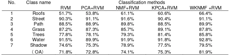
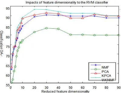
Experiment with feature extraction algorithm, feature dimensions taken before 15 feature components as input, the energy of the total energy accounted for more than 96%. The classification result was shown as Table 1, Table 2 and Table 3. An impact of feature dimensionality to the RVM classier for hyperspectral remote sensing image was shown as Figure 2 (10% training sample data).
Table 1. Classification results use 1% training sample data
No. Class name Classification methods
RVM PCA+RVM NMF+RVM KPCA+RVM WKNMF +RVM
1 2 3 4 5 6 7 Roofs Street Path Grass Trees Water Shadow 51.7% 90.3% 88.5% 87.2% 77.8% 91.5% 74.6% 53.8% 91.1% 88.9% 87.3% 78.1% 89.9% 75.3% 61.1% 91.6% 89.8% 85.7% 79.3% 91.9% 78.9% 60.6% 90.4% 88.5% 89.1% 81.4% 91.8% 77.5% 66.4% 91.1% 89.9% 87.8% 85.8% 92.8% 79.5%
OA 71.8% 72.8% 74.1% 75.3% 81.9%
Table 2. Classification results use 3% training sample data
No. Class name Classification methods
RVM PCA+RVM NMF+RVM KPCA+RVM WKNMF +RVM
1 2 3 4 5 6 7 Roofs Street Path Grass Trees Water Shadow 55.1% 91.5% 89.5% 87.5% 78.8% 91.2% 78.6% 56.7% 91.2% 88.9% 88.3% 80.1% 91.9% 79.3% 62.3% 92.3% 94.6% 89.7% 85.1% 93.3% 81.9% 62.2% 92.4% 95.5% 92.5% 86.4% 93.8% 81.3% 68.6% 93.1% 95.9% 94.8% 86.8% 95.8% 83.2%
OA 74.8% 75.8% 77.8% 78.8% 82.3%
Table 3. Classification results use 5% training sample data
No. Class name Classification methods
RVM PCA+RVM NMF+RVM KPCA+RVM WKNMF +RVM
1 Roofs 61.1% 63.8% 66.5% 70.1% 76.7%
2 Street 97.5% 100% 93.4% 96.4% 95.5%
3 Path 99.5% 99.9% 100% 98.5% 99.9%
4 Grass 97.2% 97.3% 96.7% 100% 97.2%
5 Trees 97.8% 97.1% 98.3% 93.4% 93.4%
6 Water 100% 98.9% 96.9% 95.8% 96.8%
7 Shadow 81.6% 78.3% 84.9% 87.5% 84.8%
Figure 2. Classification OA with respect to reduced dimensionality in HYDICE (10% training sample data)
3.2. Experimental on AVIRIS Data Set
The experiments were carried out on HSI images produced by the AVIRIS. In order to simplify the logistics of marking this example analysis available to others, only a small portion of data set was chosen for this experiment. It contains 145 lines by 145 pixels (21025 pixels) and 190 spectral bands selected from a June 1992 AVIRIS data set of a mixed agriculture/forestry landscape in the Indian Pine Test Site in Northwestern Indiana.
We select corn-min, corn-notil, soybean-min, soybean-notil and woods from AVIRIS images for classification experiment. The 3-bands (20, 80, 140 band) false color synthesis image used in experiment and the ground truth are shown in Figure 3.
Figure 3. False color images and ground truth of AVIRIS
Classification experiments on hyperspectral data with RVM, PCA+RVM, NMF+RVM and KPCA+RVM (Gauss kernel, width coefficient is 0.5) respectively, compared with the KNMF+RVM method proposed in this paper. The Overall Accuracy (OA) used as evaluation stand in the experiment results. Experiment randomly select 0.5%, 2% and 5% samples respectively as training data sets on original hyperspectral data and other samples as test data sets. The classification experiments were repeated 10 times as HYDICE experiment, taking the statistical average for final results. The RVM kernel functions are used RBF (Radial Basis Function) kernel function, the width coefficient of 0.5.
Table 4. Classification results use 0.5% training sample data
No. Class name Classification methods
RVM PCA+RVM NMF+RVM KPCA+RVM WKNMF +RVM
1 corn-min 73.3% 74.3% 75.1% 76.6% 78.4%
2 corn-notil 70.9% 71.7% 72.4% 75.4% 81.1%
3 soybean-min 77.6% 78.3% 80.6% 83.5% 89.9%
4 soybean-notil 52.5% 54.3% 56.0% 59.1% 63.8%
5 Woods 85.6% 87.1% 89.6% 89.4% 90.8%
OA 68.6% 70.0% 71.5% 73.3% 76.7%
Table 5. Classification results use 2% training sample data
No. Class name Classification methods
RVM PCA+RVM NMF+RVM KPCA+RVM WKNMF +RVM
1 corn-min 77.4% 77.6% 77.7% 80.6% 83.4%
2 corn-notil 76.3% 75.5% 77.8% 79.4% 82.1%
3 soybean-min 83.5% 83.7% 83.8% 88.5% 90.1%
4 soybean-notil 57.9% 58.8% 60.7% 65.1% 67.8%
5 Woods 91.1% 91.2% 92.3% 93.4% 95.8%
OA 73.2% 74.2% 75.1% 77.3% 80.5%
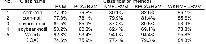
Table 6. Classification results use 5% training sample data
No. Class name Classification methods
RVM PCA+RVM NMF+RVM KPCA+RVM WKNMF +RVM
1 corn-min 77.9% 79.8% 80.1% 82.6% 86.1%
2 corn-notil 77.3% 78.1% 79.9% 81.4% 85.6%
3 soybean-min 84.5% 85.9% 87.2% 89.5% 93.9%
4 soybean-notil 58.2% 60.3% 62.4% 69.1% 73.8%
5 Woods 92.8% 93.4% 94.0% 94.4% 95.8%
OA 74.6% 75.9% 77.4% 79.3% 84.8%
From the classification experimental results, it can be seen that the application of the proposed method is better than the other algorithms, and the performance of wavelet kernel function is superior to the traditional kernel function. The classification accuracy using RVM classifier can achieve higher with fewer samples, hyperspectral image classification problems so it is suitable for small sample, high dimension and large amount of data.
4. Conclusion
A novel kernel framework for hyperspectral image classification based on RVM is presented in this paper. This WKNMF method uses the kernel function into the NMF and improved it by Mexican hat wavelet kernel function. By the feature of multi-resolution analysis, the nonlinear mapping capability of WKNMF method can be improved. Because of RVM has good generalization ability, difficult affected by the classifier parameters selection and in the choice of regularization coefficient appropriate, RVM has approximate classification accuracy as SVM. So we combine WKNMF and RVM as new classification framework for HSI data.
The experiment on HYDICE and AVIRIS data sets show that the WKNMF method as feature extraction has more ability than the compared algorithms, and the performance of wavelet kernel function has better performance than general kernel function. The final processed data is applied to HSI image classification based on RVM classifier. In some cases, the classification accuracy can be increased over 10% and the classification precision can effectively improve in small sample area. Experiment results proved the effectiveness of the classification framework.
Acknowledgements
References
[1] J Muñoz-Marí, D Tuia, G Camps-Valls. Semisupervised classification of remote sensing images with active queries. IEEE Trans.on Geosci. Remote Sensing. 2012; 50(10): 3751-3763.
[2] Bioucas-Dias JM, Plaza A, Camps-Valls, G Scheunders P, Nasrabadi NM, Chanussot J. Hyperspectral Remote Sensing Data Analysis and Future Challenges. IEEE Geoscience and Remote Sensing Magazine. 2013; 1(2): 6-36.
[3] Yushi Chen, Xing Zhao, Zhouhan Lin. Optimizing Subspace SVM Ensemble for Hyperspectral Imagery Classification. IEEE Journal of Selected Topics in Applied Earth Observations and Remote Sensing. 2014; 7(4): 1295-1305.
[4] Dopido I, Villa A, Plaza A, Gamba P. A Quantitative and Comparative Assessment of Unmixing-Based Feature Extraction Techniques for Hyperspectral Image Classification. IEEE Journal of selected topics in applied earth observations and remote sensing. 2012; 5(2): 421-435.
[5] YL He, DZ Liu, SH Yi. A new band selection method forhyperspectral images. Opto-Electronic Engineering. 2010; 37(9): 122-126.
[6] F Liu, JY Gong. A classification method for high spatial resolution remotely sensed image based on multi-feature. Geography and Geo-Information Science. 2009; 25(3): 19-41.
[7] H Su, H Yang, Q Du, YH Sheng. Semisupervised band clustering for dimensionality reduction of hyperspectral imagery. IEEE Geoscience and Remote Sensing Letters. 2011; 8(6): 1135-1139. [8] Sen Jia, Yuntao Qian. Constrained Nonnegative Matrix Factorization for Hyperspectral Unmixing.
IEEE Transactions on Geoscience and Remote Sensing. 2009; 47(1): 161-173.
[9] Xuesong Liu, Wei Xia, Bin Wang, Liming Zhang. An approach based on constrained nonnegative matrix factorization to unmix hyperspectral data. IEEE Transactions on Geoscience and Remote Sensing. 2011; 49(2): 757-772.
[10] Song Xiangfa, Jiao Licheng. Classifiction of hyperspectral remote sensing image based on sparse representation and spectral information. Journal of Electronics & Information Technology. 2012; 34(2): 268-272.
[11] Fauvel M, Chanussot J, Benediktsson JA. A Spatial spectral Kernel based Approach for the Classification of Remote sensing Images. Pattern Recognition. 2012; 45(1): 381-392.
[12] Chen Yi, Nasser M, Trac DT. Hyperspectral Image Classification via Kernel Sparse Representation. IEEE Transactions on Geoscience and Remote Sensing. 2013; 51(1): 217-231.
[13] Wang J. Jabbar MA. Multiple Kernel Learning for adaptive graph regularized nonnegative matrix factorization. National association of science and technology for development. 2012; 41(3): 115-122. [14] Mahesh pal, Giles M Foody. Evaluation of SVM, RVM and SMLR for Accurate Image Classification
with Limited Ground data. IEEE Journal of selected topics in applied earth observations and remote sensing. 2012; 5(5): 1344-1355.
[15] Yunjie Xu, Shudong Xiu. Diagnostic Study Based on Wavelet Packet Entropy and Wear Loss of Support Vector Machine. TELKOMNIKA Telecommunication Computing Electronics and Control. 2014; 12(4): 847-854.
[16] Wei Feng, Wenxing Bao. A New Technology of Remote Sensing Image Fusion. TELKOMNIKA Telecommunication Computing Electronics and Control. 2012; 10(3): 551-556.
[17] FA Mianji, Y Zhang. Robust hyperspectral classification using relevance vector machine. IEEE Trans. Geosci. Remote Sens. 2011; 49(6): 2100-2112.