Extensive Tracking Performance Analysis of Classical feedback control
for XY Stage ballscrew drive system
L.Abdullah, Z.Jamaludin, Chiew T.H., N.A. Rafan, M.Y. Yuhazri
Faculty of Manufacturing Engineering, Universiti Teknikal Malaysia Melaka, Durian Tunggal, 76100 Melaka, Malaysia
Phone: +606-3316973, Fax: +606-3316411, Email: [email protected]
Keywords: Performance Analysis, XY Stage, PID controller, Frequency Domain Analysis.
Abstract. Performance analysis in term of identifying the system's transient response, stability and system's dynamical behavior in control system design is undeniably a must process. There are several ways in which a system can be analyzed. An example of well known techniques are using time domain and frequency domain approach. This paper is focused on the fundamental aspect of analysis of classical feedback controller in frequency domain of XY milling table ballscrew drive system. The controller used for the system is the basic PID controller using Matlab SISOTOOL graphical user interface. For this case, the frequency response function (FRF) of the system is used instead of using estimated model of transfer function to represent the real system. Result in simulation shows that after proper tuning of the controller, the system has been successfully being controlled accordingly. In addition, the result also fulfill the set requirement of frequency domain analysis in terms of the required gain and phase margin, the required maximum peak sensitivity and complimentary sensitivity function and the required stability.
Introduction
Accuracy and precision is decisive in machining process. However, the presence of disturbance forces leads to inaccuracy in positioning and tracking [3]. A good example of disturbance force that greatly affects tracking performance is cutting forces. Cutting force exist in nature of the milling process and simply cannot be avoided as it is generated from the contact between the cutting tool and the work piece. Kalpakjian and Schmid [8] mention that cutting force is influenced by the milling parameters such as the depth of cut and spindle speed. In literature, problem regarding cutting force in milling process have been studied extensively and many controllers have been proposed and validated. Quite a number of techniques have been introduced and recorded in [2], [3] and [7] using different techniques such as cascade P/PI, inverse-model-based disturbance observer and repetitive controller.
The classical PID controller is extensively known in many industrial applications such as temperature control of refrigerator [5] and air conditioning system [6]. Its flexibility allowed benefits from the advances of technology. It is the combination of PI and PD controller which can improve both steady state error and transient response [7]. This paper is organized as follows. Section 2 describes the experimental setup. Section 3 discusses the design of PID controller. Section 4 describes the performance analysis in frequency domain. Section 5 summarizes the main conclusions of this paper.
Experimental Setup
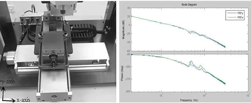
The considered system setup is a ball screw drive XY milling table as shown in figure 1. The XY milling table is produced by Googol Tech and it consists of two axes which are x and y axes. Both axes are driven by one Panasonic MSMD 022G1U A.C. servo motor and equipped with an incremental encoder for positioning measurement respectively. The resolution of the encoder is 0.0005 mm/ pulse. The length of the milling table for both axes is 300mm respectively. Two limit switches are positioned at the near end of both axes for safety purposes. The total mass for x-axis is 36.8 kg while total mass for y-axis is 23.4 kg. The FRF of each axis contains an anti-resonance and resonance combination near 47 Hz based on figure 2 that has been examined at the resonance part.
Figure 1: Ball screw drive XY milling table. Fig. 2. FRF measurements of x- and y-axes.
Design of controller
For the purpose of controlling the system, PID controller was utilized and chosen. PID controller are designed based on the identified system shown in figure 2. The second order dynamic behaviour of the system is as follows:
. . (1)
where Y is the position in millimeter and U is the input signal in voltage.
PID Controller. The general transfer function of the PID controller, showed in (2).
, (2)
where Kp, Ki, and Kd are the gain values for proportional (P), integral (I) and derivative (D)
components of the controller. The controller is designed based on traditional open loop shaping followed by closed loop tuning. Matlab sisotool graphical user interface has been fully utilized during the design stage of the parameter of the controller. The parameters of this controller are designed and tuned based on the universal rule of thumb of phase margin and gain margin. Pole zero plot and Nyquist Diagram was utilized to check for stability. Step response and Bode diagram of closed loop transfer function is used to check the transient response behaviour and bandwidth of the system. The gain value obtained for Kp, Ki, and Kd are 1.9761 volts.sec / mm, 0.002 volts.sec /
mm and 0.0988 volts.sec / mm respectively.
Performance Analysis in Frequency Domain
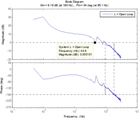
Gain & Phase Margin Analysis. Referring to table 1 and figure 3, it can be seen that the Gain Margin, Gm and Phase Margin, Pm of the open loop Controlled and Uncontrolled system are as
follows :
Table. 1. Gain and Phase Margin of open loop system
Open Loop System Gain Margin, GM Phase Margin
Uncontrolled System 25.5 dB 79 degree
Fig. 3. Open Loop Bode Diagram of PID controlled system
The Gain Margin tells how much gain can be added to the system before the system become unstable. Therefore, the higher the Gain Margin, the more gain can be added to the system however as the value of the Gain margin increases the performance in term of the speed response will be reduced [4]. In general, it is desired to be in the range of Gain margin between 4dB to 10dB in order to preserve better performance in term of the speed response. It is proven that the tuned system is within the desired range of gain margin. Next, the Phase Margin tells how much negative phase (phase lag) can be added to the system, L(s) at frequency, Wc before the phase at this frequency becomes -180 degree which corresponds to closed loop instability. The concept is the same like gain margin in which the higher the value of the phase margin the more phase lag can be added to the system, but the speed response will be reduced if the value of the phase margin is too high [1]. So, the rule of thumb for phase margin is to get the value within the range of 30 degree to 90 degree. Therefore, the tuned system is also within the desired range of phase margin.
Fundamental of Loop Shaping and Gain Crossover Frequency Analysis. Gain crossover frequency is the frequency where |L(jwc)|first crosses magnitude 1 (or 0 dB line) from above [4]. Referring to table 2, it shows that the value of Gain crossover frequency of uncontrolled and PID controlled system are as follows
:-Table. 2. Gain crossover frequency of open loop system Real Plant,
Design of open loop system is most critical in the crossover region between crossover frequency, Wc. In order to maintain stability, |L(jw180)| < 1. It simply means that the graph of L must be lower than 0 dB line at -1800. Next, in order to get fast response, it is required to have Wc and w180 large
and phase lag in L to be small [4]. Based on the value shown below, the tuned system satisfy all of it. Thirdly, in order to get the maximum benefit of feedback control, it is desired to have a loop gain, L to be as large as possible within the bandwidth region. For this case, it can be seen that after the system has been tuned, the loop gain, L have been increases significantly, thus it is larger compared to the uncontrolled system. For the case of real plant, to be exact, the loop gain, L of the tuned system is above 0 dB line from frequency equivalent to 0.1 Hz until at least almost at the frequency of bandwidth which is 44.6 Hz, whereas the loop gain ,L of the uncontrolled system is above 0 dB line from 0.1 Hz until 5.45 Hz only. Thus, it proves that the loop gain, L of the tuned system is larger than the loop gain of uncontrolled system.
Bandwidth Analysis. Bandwidth frequency of a system is a measure of performance of a system in terms of dynamical behaviour like speed response. In general, the higher the bandwidth of the system the better the system is. Bandwidth can be divided in two different type of categories. Firstly, it is called close loop bandwidth, WB. It can be defined as the frequency where the
sensitivity function of the system first crosses at -3 dB line. Secondly, it is called complimentary bandwidth, WBT. As the name implies, Complimentary bandwidth frequency is the frequency where
the complimentary sensitivity function of the system first crosses at -3 dB line [4],[9]. Referring to Table 3, it shows that the Bandwidth of the close loop PID Controlled and Uncontrolled system for the real plant are as follows
:-Table 3. Bandwidth of the PID controlled and uncontrolled system
Close Loop System Close Loop Bandwidth, WB Complimentary
Bandwidth, WBT
Uncontrolled System 4.77 Hz 6.82 Hz
PID controlled system 45.4 Hz 80.4 Hz
Theoretically, for systems with Pm < 900, the result will be WB < WC < WBT . It is proven using
this case in which Pm = 540 , WB = 45.4 Hz , WC = 44.6 Hz and WBT = 44.8 Hz. As a result, WB
< WC < WBT and thus it proved the theory. From the result, it is known that up to frequency of
45.4 Hz which is the close Loop Bandwidth the control of the system is effective in terms of improving performance whereas in the frequency range above 45.4 Hz in which Sensitivity of the system above 0 dB line, the control has no significant effect to the response. In other words, it is better to run the system within the system frequency bandwidth up to 45.4 Hz only.
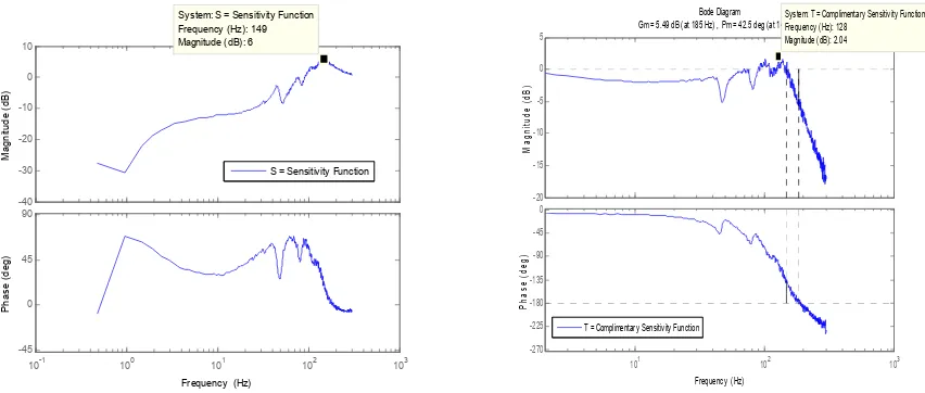
Maximum Peak Sensitivity and Complimentary Sensitivity Analysis. Maximum Peak Sensitivity Function, Ms is the maximum value in magnitude of the bode diagram of sensitivity function. In order to get better frequency domain performance, the required maximum peak for the sensitivity function must be less than or equal to 6 dB [4]. Based on figure 4, it is shown that the maximum peak sensitivity is equal to 6 dB. Thus, the tuned system do satisfy the requirement of the maximum peak criteria. Furthermore, the peak at 6 dB only occurred at frequency of 149 Hz which is beyond the closeloop bandwidth frequency and since the system will be run only within the range of the system bandwidth, thus it does not affect the performance of the system. Notes that if maximum peak sensitivity, Ms is above 12 dB line, it indicates that the system is poor in term of performance and poor in term of robustness [4].
Maximum Peak Complimentary Sensitivity Function, MT is the maximum value in magnitude of
the bode diagram of complimentary sensitivity function [4]. In order to get better frequency domain performance, the required maximum peak for the complimentary sensitivity function must be less than 2 dB. Referring to figure 5, it shows that the maximum peak complimentary sensitivity is equal to 2.04 dB. Thus, the tuned system do satisfy the requirement of the maximum peak criteria. Furthermore, the peak at 2.04 dB only occurred at frequency of 128 Hz which is beyond the closeloop bandwidth frequency and since the system will be run only within the range of the system bandwidth, thus it does not affect the performance of the system. Notes that if maximum peak complimentary sensitivity, MT is above 12 dB line, it indicates that the system is poor in term of
Fig. 4. Max. Peak Sensitivity Function ( = 6dB)
Fig. 5. Max. Peak Complimentary Sensitivity Function ( = 2dB)
Stability and Tracking Error Analysis. Referring to figure 7, it is shown that the close loop real plant is stable since the close loop system does not encircle at s = -1. In theory, in order to maintain close loop stability, the number of encirclements of the critical point -1 by open loop, L (jw) must not change[4]. In other words, it is required that open loop, L (jw) to stay away from this point. On the other hand, the modulus margin, Ms-1 is the smallest distance between L(jw) and -1. Thus, in order to obtain robust stability, it is required for the control designer to obtain smaller value of the maximum peak sensitivity. In other words, the smaller the value of the maximum peak sensitivity , the better robust stability condition of the system will be. However the disadvantages of having too much robust stability is the system will have slower performance in term of speed response[4],[9].
For this case, the value of modulus margin is roughly about 0.544. Since the distance modulus margin is small it does represent that the system have a very fast response with the stability of the system still being preserved because the value of modulus margin is not zero. When the value of modulus margin is less or equal to zero, it represent that the system is no longer stable. On the other hand, based on figure 6, it is found that the Tracking Error for this case is 0.2247 mm. It simply means that after travelling for supposedly 15mm that is set as a desired position, the system actual final position is 14.7753 mm.
Fig. 6. Tracking performance of the system Fig. 7. Nyquist Diagram of the PID controlled system
10-1 100 101 102 103
0 500 1000 1500 2000 2500 3000 3500 4000 4500
Conclusion
In conclusion, in order to quantify the performance of the system in frequency domain using any type of classical controller, there are certain requirements or guidelines that is advisable to be accomplished by the control system designer. Those requirements are phase and gain margin requirement, gain crossover frequency, bandwidth, maximum peak sensitivity and complimentary sensitivity and stability requirement. Result shows that the controller has been successfully fulfilled all the desired requirement as mentioned in the theory.
References
[1] G.F. Franklin, J.D.Powell, A.E Naeni, "Feedback control of dynamic systems" Singapore: 6ed., Pearson Prentice Hall, 2010.
[2] Z. Jamaludin, H. V. Brussel, G. Pipeleers and J. Swevers, “Accurate Motion Control of XY High-Speed Linear Drives using Friction Model Feedforward and Cutting Forces Estimation”.
CIRP Annals – Manufacturing Technology, Vol. 57, Issue 1, pp. 403-406, 2008.
[3] Z. Jamaludin, H. V. Brussel and J. Swevers, “ Classical Cascade and Sliding Mode Control Tracking Performances for a XY table of a High-Speed Machine Tool”. International Journal of Precision Technology, Vol. 1, No. 1, pp. 65-74, 2007.
[4] S. Skogestad and I. Postlewaite, "Multivariable Feedback Control: Analysis and Design". Singapore: Wiley, 2005.
[5] N. H. Abdul Hamid, M. M. Kamal and F. H. Yahaya, “ Application of PID Controller in Controlling Refrigerator Temperature”. 5th International Colloquium on Signal Processing & Its Applications (CSPA) (6 – 8 Mar 2009 – Kuala Lumpur, Malaysia), pp. 378-384.
[6] M. Du, Z. Zhang and Y. Liu, “A Research on Expert Fuzzy – PID Fusion Controller Algorithm in VAV Central Air Conditioning System”. Third International Symposium on Intelligent Information Technology Application (IITA) (21 – 22 Nov 2009 – NanChang, China), pp. 194-198.
[7] Z. Jamaludin, Disturbance Compensation for a Machine Tools with Linear Motors. Ph. D. Dissertation, Department Wertuigkunde Katholieke Universiteit Leuven, Belgium, 2008.
[8] S. Kalpakjian and S. Schmid, "Manufacturing Engineering and Technology". Singapore: Pearson Prentice Hall, 2006.