DETECTING ANOMALY REGIONS IN SATELLITE IMAGE TIME SERIES BASED ON
SESAONAL AUTOCORRELATION ANALYSIS
Z.-G. Zhou a, P. Tang b, *, M. Zhou a
a Academy of Opto-electronics (AOE), Chinese Academy of Sciences (CAS), Beijing 100094, China; Key Laboratory of Quantitative Remote Sensing Information Technology, CAS – (zgzhou, zhoumei)@aoe.ac.cn b Institute of Remote Sensing and Digital Earth (RADI), Chinese Academy of Sciences (CAS), Beijing 100101, China –
Commission III, WG III/3
KEY WORDS: Anomaly Detection, Remote Sensing, Disturbance Detection, SARIMA, Temporal Autocorrelation, Time Series
ABSTRACT:
Anomaly regions in satellite images can reflect unexpected changes of land cover caused by flood, fire, landslide, etc. Detecting anomaly regions in satellite image time series is important for studying the dynamic processes of land cover changes as well as for disaster monitoring. Although several methods have been developed to detect land cover changes using satellite image time series, they are generally designed for detecting inter-annual or abrupt land cover changes, but are not focusing on detecting spatial-temporal changes in continuous images. In order to identify spatial-temporal dynamic processes of unexpected changes of land cover, this study proposes a method for detecting anomaly regions in each image of satellite image time series based on seasonal autocorrelation analysis. The method was validated with a case study to detect spatial-temporal processes of a severe flooding using Terra/MODIS image time series. Experiments demonstrated the advantages of the method that (1) it can effectively detect anomaly regions in each of satellite image time series, showing spatial-temporal varying process of anomaly regions, (2) it is flexible to meet some requirement (e.g., z-value or significance level) of detection accuracies with overall accuracy being up to 89% and precision above than 90%, and (3) it does not need time series smoothing and can detect anomaly regions in noisy satellite images with a high reliability.
1. INTRODUCTION
Anomaly is a pattern in the data that does not conform to the expected behaviour, also referred to as outliers, exceptions, peculiarities, surprises, etc. (Chandola et al., 2009). Anomalies in satellite images can translate to significant land cover changes or disturbances, which may be caused by nature (e.g., fire, flood, severe drought, and windstorm), biogenic factors (e.g., plant diseases, insect pests) or anthropogenic activities (e.g., deforestation, urbanization) (Hecheltjen et al., 2014; Verbesselt et al., 2012).
Anomaly regions in satellite images can reveal land cover changes or disturbances occurring worldwide at unknown time and location. Satellite image time series possess significant potential for monitoring land cover changes at regional to global scales, due to the synoptic and frequent satellite observation (Hansen and Loveland, 2012). Satellite image time series from the AVHRR (Advanced Very High Resolution Radiometer), MODIS (MODerate-resolution Imaging Spectroradiometer) and the coming Sentinel Constellation, for instance, provide consistent observation of land cover over large areas and at high frequencies. Satellite image time series continuously records the varying status of land cover, including the seasonal patterns driven by annual temperature and rainfall interactions, as well as the anomalies caused by anthropogenic or natural factors (Verbesselt et al., 2012).
Detection of anomaly regions in satellite image time series is important for researchers to study the dynamic processes of land cover changes, as well as for resource managers to monitor land cover dynamics over large areas, especially where access is
* Corresponding author
difficult or hazardous (Kennedy et al., 2009; Pickell et al., 2014). Long term satellite image time series has been used to detect anomaly region for identifying land cover changes or disturbances (Lu et al., 2004). A challenge in anomaly region detection in satellite image time series is to understand what constitutes anomalies amidst background seasonal variation (Hutchinson et al., 2015; Verbesselt et al., 2012).
However, although these methods can, to some extent, get promising results of anomaly region detection in satellite image time series, they are generally designed for detecting inter-annual land cover changes or occurrence of abrupt changes in the time series. In order to more comprehensively identify and characterize the dynamic processes of spatial-temporal changes of land cover (e.g., intra-annual changes), it is practical to develop a method for detecting anomaly regions in each image of satellite image time series.
To this end, this paper proposes a method that is based on seasonal autocorrelation analysis of time series data, for detecting anomaly regions in each image of satellite image time series. The method is composed of two steps: (1) anomaly enhancement by seasonal autocorrelation analysis based on a Seasonal Autoregressive Integrated Moving Average (SARIMA) model (Cryer and Chan, 2008), and (2) anomaly detection using a criterion based on statistical analysis of anomaly-enhanced time series data. The method is tested with a case study for detecting anomaly regions caused by severe flooding (i.e., detecting anomalous flood areas) occurred at the border of southeast Russia and northeast China in 2013. The test data is Normalized Differencing Vegetation Index (NDVI) image time series from the satellite Terra/MODIS and the reference data is multi-spectral ETM+ and OLI images from the satellite Landsat. Experiment results demonstrate the effectiveness of the proposed method that it can detect anomaly regions in each image of the MODIS NDVI image time series, with overall accuracy being up to 89%.
This paper is organized as follows. Section 2 simply introduces the principle of seasonal autocorrelation analysis of time series using SARIMA model. Section 3 describes how to enhance and further to determine anomaly region in satellite image time series using a SARIMA model and a statistical analysis criterion. In section 4, the method is demonstrated with the case study for detecting anomaly regions caused by big flooding, followed by a conclusion of this paper in Section 5.
2. SEASONAL AUTOCORRELATION ANALYSIS
2.1 SARIMA Model for Autocorrelation Analysis
In a time series, any data is correlated to others in the same time series, with correlation coefficient being from zero to one. This kind of correlation of the data within time series is well known as autocorrelation. From this point of view, a seasonal time series can be represented with a Seasonal Autoregressive Integrated Moving Average (SARIMA) model (Cryer and Chan, 2008), which is a common model for analysing autocorrelation of seasonal time series data.
Given a seasonal time series Y with period s, where t is an integer time index and the Y are real numbers, then a SARIMA model can be given by:
= autoregressive (AR) part with order p, ( )L order Q of the SARIMA model
In the SARIMA model in Equation 1, the d t Y
and D t sY
are
respectively the differencing term with degree d and the seasonal differencing term with degree D:
and the error terms
ε
are generally assumed to be independent, identically distributed variables sampled from a normal distribution with zero mean. The SARIMA model is generally denoted as:SARIMA( , , ) ( , , )p d q P D Q S (4) where s refers to the number of seasons/data in a period/cycle, the parameters p, d, q, P, D and Q are non-negative integers refer to the orders/degrees of the model, as shown in Equation 2 and 3. If a time series does not have seasonal variation, the parameters P, D and Q of the seasonal part of the SARIMA model would be zeros.
2.2 Seasonal Autocorrelation of Satellite Time Series
The varying pattern of a satellite time series Y (see Figure 1(a) as an example) can be well fitted and represented with a SARIMA model with proper parameters. In practice, however, anomalous data in the satellite time series may also be falsely fitted with that SARIMA model, resulting in miss of anomaly detection. Nevertheless, the point in question is not the varying pattern of time series to represent, but the anomalies in the time series to detect. For this purpose, one should exploit appropriate parameters of SARIMA model to extract or enhance anomalies in the satellite time series, other than to well fit the varying pattern of satellite time series.
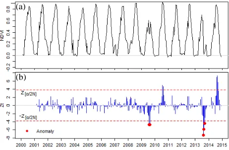
Figure 1. (a) NDVI time series data. (b) Anomaly-enhanced time series data, z, and the detected anomalies (red dots).
In principle, seasonality characterizes the satellite time series to some extent (from slight to strong). As shown in Figure 1(a),The time series data from satellite images has clear seasonal varying pattern because the vegetation phenology is highly impacted by annual temperature and rainfall (Verbesselt et al., 2012). Here,
(a)
we assume that the satellite time series data has linear trend or no trend (otherwise, the trend can be removed beforehand using yearly average or Seasonal-Trend Decomposition based on Loess (STL) for example). Under normal conditions, the status of land cover in a period (e.g. September) in a year would be similar to those in the same period in other years. That is to say that the satellite time series data is strongly seasonal autocorrelated. Since only the anomalies in the satellite time series are of interests but the temporal varying patterns are not, here only the seasonal autocorrelation of satellite time series (representing seasonality) is considered but the non-seasonal autocorrelation of satellite time series is not. The seasonal autocorrelation of a time series can be represented by:
SARIMA(0,0,0) ( , , ) P D Q S (5)
i.e., only the parameters for seasonal part of the SARIMA model are left and those for non-seasonal part are all set to be zeros.
3. ANOMALY REGION DETECTION
Anomaly region is detected from satellite image time series pixel by pixel. Based on the fact that the anomalies in satellite time series data are those not conformed to the expected seasonal pattern, and the fact that the satellite time series data is seasonal auto-correlated, a practical way to distinguish the anomalies from the seasonal pattern is to remove the seasonality of the time series, via the seasonal autocorrelation analysis. What is more, since anomalies are mixed with erratic fluctuations (i.e., noises) in satellite time series, anomalies can be determined with some criterion based on statistical analysis.
3.1 Anomaly Enhancement by Seasonal Autocorrelation Analysis
A practical way to remove the seasonality of satellite time series data is first degree seasonal differencing (seasonal differencing, for short) (Cryer and Chan, 2008), even if there is slight or no seasonal pattern in the time series. The seasonal differencing of the time series Y , � �, can be denoted as:
� � = SARIMA , , × , , s (6)
where the parameters P and Q are given zeros. This is because it is hypothesized here that for satellite time series data, a data at a period in a year is strongly correlated with the data at the same period in other years. This is to say, under normal condition, the status of land cover in this year is similar to the status in other years at the same season or time period.
If there is no anomaly in satellite time series data, the differences between the data of adjacent years, i.e., � �, would be random noises, denoted ε . It is assumed to be independent and identically distributed variables sampled from a normal distribution with mean μ and variance σ2. Then, the seasonal differencing of time series would be ε. Otherwise, if there is an anomaly with magnitude m at time t, it might be extracted by subtracting the random noise from the seasonal difference time series:
m = ∇ Y − ε (7)
In practice, however, one does not known the prior knowledge of the distribution of random noise ε. A general way to estimate the noise term is to suppose there is no anomaly in the time series data. Since the time series data as well as the probably anomalies may have different magnitudes, the seasonal differenced time series is normalized to near standard normal distribution, for
simplicity to determine anomalies from noises. Here, the anomaly-enhanced time series, denoted �, is defined as:
� = � � − � /� (8)
where � = mean value of the seasonal differenced time series
� = / 2 sYt , robust standard deviation (Cryer and Chan, 2008) of the seasonal differenced time series.
Then, the anomalies in a satellite time series would be obvious in the anomaly-enhanced time series, which is assumed to follow standard normal probability distribution. See Figure 1(b) for an illustration of the anomaly-enhanced time series z.
3.2 Criterion for Anomaly Determination
The anomaly-enhanced time series z contains information of both anomaly m and noise ε. If a time series Y has exactly one anomaly at time T, then ∇ YT= εT+ mT but ∇ Y = ε otherwise. Therefore, the z has (approximately) a standard normal distribution under the null hypothesis that there is no anomaly in the time series (Cryer and Chan, 2008).
When T is known beforehand, the observation is declared an anomaly at the 5% significance level (α = . 5) if the corresponding z exceeds a threshold of 1.96 (i.e., the z-value
z[0.05/2]) (Cryer and Chan, 2008). In practice, however, there is often no prior knowledge about the number and the time of anomalies. To detect anomalies, the test of z should be applied to all observations in the time series. In the process of detection, the threshold of 1.96 for z would result in 5 anomalies in 100 tests just by chance, even if there is actually no anomaly (Cryer and Chan, 2008). A simple and conservative way is to use the Bonferroni Correction for controlling the overall error rate of multiple tests of anomalies (Cryer and Chan, 2008). An observation could be tentatively identified as anomaly if the corresponding z exceeds the upper . 5/ N × % percentile of the standard normal distribution (N is the length of time series). This way can greatly reduce the probability (e.g., at most a 5% probability if α = . 5) of false detection of anomalies in the whole time series data (Cryer and Chan, 2008).
Therefore, to detect anomalies at a significance level α, an observation at time t could be tentatively identified as anomaly if
|z | > z[α/2N], where the z[α/2N] is the z-value that meets:
P(|z| > z[α/2N]) = α/ N (9)
However, an anomaly in the anomaly-enhanced time series at time t-s (s is the period of the time series), m− , would be affect the anomaly-enhanced time series at time t (see Figure 1(b) for illustration). This is because if Y− = Y−2 + ε− + m− , then
∇ Y = Y − Y− = Y − Y−2 − ε− − m− ≈ −ε− − m−. Thus, −m− would be a fake anomaly at time t.
Therefore, to determine anomalies from the anomaly-enhanced time series and to filter out fake anomalies, a criterion of anomaly detection is defined:
|� | > �[�/2�] ��� |�−| ≤ �[�/2�] (10)
4. EXPERIMENTS AND RESULTS
4.1 Materials
4.1.1 Case Study Area: The study area is around a border of southeast Russia and northeast China, with the Heilongjiang River being as the border of two countries (see Figure 2(a), Russia to the north and China to the south). The geographic coordinates of the study area are “133.4255E, 48.4654N” for the north-west corner and “134.7849E, 48.0569N” for the south-east corner, covering about 6,000 km2 with roughly 120 km by 50 km
In the study area, main types of land cover include forest, shrub, urban and water. From the year 2000 to 2015, the land cover types are consistent over years and there is no significant changes of land cover types. However, a big flood occurred in the summer of 2013 and the river broke through its banks on August 23, causing severe flooding over large areas for as long as two months (see Figure 2(a-e)).
The Heilongjiang River is a seasonal river, i.e., it has seasonal floods in each year and it has different water areas in different seasons. Normal flooding in riverbank during the summer should not be seen as unexpected land cover disturbance. However, severe flooding caused inundation over towns and farmlands around the river during the summer of 2013. The unexpected flooded region during this period should be taken as anomaly region.
4.1.2 Satellite Image Time Series: The 16-day composited MODIS vegetation indices products (MOD13Q1) provide image time series (23 images per year, s=23 for Equation 10) with medium-coarse spatial resolution (250 meter) and low cloud-contamination. The MOD13Q1 products covering the study area from February 2000 to February 2015 (345 images in total) were collected from the LAADS (http://ladsweb.nascom.nasa.gov). There are 609×183=111447 pixels in each image. In Figure 2 , the subtitle of each image indicates the 16-day composited period of the MODIS NDVI image.
The NDVI image time series from the satellite Terra/MODIS was selected as test data. Since NDVI is a commonly used indicator of vegetation status, and different types of land covers have distinct NDVI values at different time (Defries and Townshend, 1994; Loveland et al., 2000), special temporal changing pattern would reside in the NDVI time series data in the case of flooding. If vegetation areas or other non-water areas are flooded unusually, the NDVI time series values will decrease dramatically and will be much lower than those in previous years. The use of Normalized Difference Water Index (NDWI) would be better to reproduce a clearer land-water separation, but when compared to NDVI, it may be less appropriate to reveal the varying pattern of vegetation and the NDWI data derived from MODIS product has coarser spatial resolutions (i.e., 500-meter).
4.1.3 Reference Images: Some contemporary satellite images with higher spatial resolution (30 meter) were selected as reference images. The multi-spectral Enhanced Thematic Mapper Plus (ETM+) images from the satellite Landsat-7 and OLI images from the satellite Landsat-8 covering the study area from 2012 to 2013 were collected from the Earth Explorer (http://earthexplorer.usgs.gov). The observing date of the reference images during the severe flooding are 2013/09/18 and 2013/09/27, which are in the Sep. 14 – Sep. 29 compositing period of the MODIS NDVI images (see Figure 2(d)).
Due to the failure of the Scan Line Corrector (SLC) in the ETM+ instrument since 2003, the collected ETM+ images show wedge-shaped gaps. In this study the gaps were filled by the phase 2 gap-filling algorithm (USGS, 2004). In addition, after precisely geometric correction, the four reference images were subset and re-projected to the same geographical region with the MODIS NDVI images.
To validate the results of anomaly detection from MODIS NDVI image time series, a reference map of anomaly region from the reference images was produced. At first, for distinct classes in each image (i.e., water, forest, cropland, vegetative wetland, built-up area, cloud and cloud shadow, residual gaps), we visually selected more than 5% pixels in each class as sample data. Then, each of the four images is classified using a supervised classification method Support Vector Machine (SVM) (Pal and Mather, 2005), resulting in two water maps for the year 2012 and 2013. Finally, the reference anomaly region was derived from the two water maps by subtracting the water map in 2012 from the water map in 2013. The reference images before 2012 were not used here because there was not big flood for this period so that we use the image in 2012 to represent all the images before 2012.
4.2 Results
Two experiments were conducted on the whole MODIS NDVI image time series (i.e., 345 images) using the proposed method. Anomaly regions were detected from the images pixel by pixel (111447 pixels in total) based on the above mentioned procedures, i.e., anomaly enhancement and anomaly determination. The difference of the two experiments is that the one takes a user-specified z-value of the anomaly determination criterion but the other takes varying z-values.
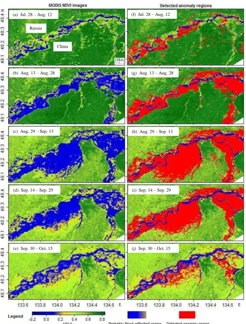
For the first experiment, the z-value was set to be two. Since the aim of the experiments was to detect anomaly regions caused by the big floods in 2013 in the case study area, the experiments results during the flooding season are shown in Figure 2. The images on the left column of Figure 2 are pseudo-coloured MODIS NDVI images, illustrating the spatial-temporal changes of big flooding from July to October in 2013. Correspondingly, the images on the right column of Figure 2 are the detected anomaly regions pasted on the NDVI images, showing the detected anomaly regions in each NDVI image.
Figure 2. The MODIS NDVI image time series (left column, a-e) showing the dynamic changes of the probably flood-affected regions in 2013, and the corresponding detected anomaly regions (right column, f-j) when setting the z-value to be two. The subtitle of each image indicates the 16-day composite period of the corresponding MODIS NDVI image.
(a) Jul. 28 – Aug. 12
(b) Aug. 13 – Aug. 28
(c) Aug. 29 – Sep. 13
(d) Sep. 14 – Sep. 29
(e) Sep. 30 – Oct. 15
(f) Jul. 28 – Aug. 12
(g) Aug. 13 – Aug. 28
(h) Aug. 29 – Sep. 13
(i) Sep. 14 – Sep. 29
(j) Sep. 30 – Oct. 15 Russia
Detected region
Reference region
Anomaly Non-
anomaly Total User Acc.
Anomaly 35094 3632 38726 90.62 %
Non-anomaly 8985 63736 72721 87.64 %
Total 44079 67368 111447
Prod. Acc. 79.62 % 94.61 %
Overall Acc. 88.68 %
Table 1. Confusion matrix of the detection results in Figure 2(i) in comparison with the reference anomaly region.
To quantitatively validate the results of the detected anomaly regions, the detection results in Figure 2(i) were compared with the reference anomaly region. Table 1 shows the confusion matrix of the comparison, including the region pixel counts and different aspects of accuracies. The Prod. Acc. (producer accuracy, a.k.a. recall or true positive rate) of the detected anomaly region is 79.62%, indicating that near four fifth of pixels in the reference anomaly region are identified as anomaly region in the MODIS NDVI image. The User Acc. (user accuracy, a.k.a. precision or positive predictive value) of the detected anomaly region is 90.62%, indicating that over nighty percent of the detected anomaly region appear in the reference anomaly region, i.e., nearly ten percent are false detections when compared to reference anomaly region. The Overall Acc. (overall accuracy) of the detected anomaly region is 88.68%, which shows that nearly nighty percent of the whole image region are correctly identified as anomaly region and non-anomaly region.
For the second experiment, the z-values of the anomaly determination criterion were continuously selected from zero to five with a 0.01 step (i.e., 600 z-values). The purpose of this experiment was to validate the detection results under different constraints in detection. The validations were also conducted by comparing the anomaly region detected from the MODIS NDVI image as shown in Figure 2(d) with the reference anomaly region.
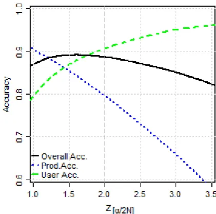
Figure 3 illustrates the curves of the anomaly region accuracies with respect to different constraints of detection (i.e., z-values of the anomaly determination criterion). The vertical grey dashed line at z=2.0 in Figure 3 just indicates the case of the first experiment. The accuracies in this specific case are just as those in the Table 1. It can be seen in Figure 3 that z=2 corresponds to neither best Prod. Acc., nor best User Acc., nor best Overall Acc. In Figure 3, when the z-value is set to be 1.0, the detection results get highest Prod. Acc. being about 91% but worst User Acc. being only about 78%. In contrary, when the z-value is set to be 3.5, the detection results get worst Prod. Acc. less than 60% but highest User Acc. more than 95%.
There is no best z-value because there are trade-offs between Prod. Acc. and User Acc. When z-value varies, the rise of the Prod. Acc. is accompanied by the decrease of User Acc., and vice versa. Nevertheless, in this experiment, the Overall Acc. are relatively stable within a small range from 83% to 90% even for a wide range of z-values.
Figure 3. The accuracies of anomaly regions detected at varying z-values of the anomaly determination criterion.
4.3 Discussion
4.3.1 Effectiveness of the Anomaly Detection Method: The first advantage of the proposed anomaly detection method is that it can effectively detect anomaly region in each image of the satellite image time series, so that it can represent spatial-temporal changes of anomaly events on land cover. As is shown in Figure 2(f-j), the detected anomaly regions in each image can show the coming and the spreading of the flood, the large area flooding after the break of riverbank, and the receding of the flood. This demonstrates that the method is able to detect spatial-temporal changing anomaly regions in the image time series. Moreover, the frequently changing areas in the images can be effectively excluded from anomaly regions. The proposed method is not compared to others here because at present few methods focus on detecting anomaly regions in each image of the satellite image time series but some methods consider detecting main disturbances/ structural changes (e.g. (Verbesselt et al., 2010b)) or occurrence of disturbance (e.g., (Zhu et al., 2012)) in satellite image time series.
The second advantage of the method is that it can be tuned according to the requirement of different aspects of accuracies. As is shown in Figure 3, on one hand, the method could result in relatively good overall accuracies (i.e., 83% to 90%) for a wide range of z-values. On the other hand, the method could get higher producer accuracy up to 90% (i.e., detect more anomaly regions) at a smaller z-value and get higher user accuracy up to 95% (i.e., more corrective anomaly regions) at a larger z-value. This demonstrates that the method is flexible and it can get satisfactory results with a reasonable z-value.
There is also a benefit of the method that it does not necessarily require time series smoothing. For one thing, smooth the satellite time series data may cause the loss of anomalies because they are generally taken as noise in many time series smoothing methods. For another, the probable anomalies in the satellite time series data could be enhanced and determined based on statistical analysis, to confidently differentiate anomalies from noise, as is shown in the example in Figure 1(b).
can be tuned to meet the user’s requirement of accuracies. The method does not need the data processing of smoothing and might be able to detect anomaly regions in noisy satellite image time series with high reliability.
However, the method also has two limitations. The one is that although data smoothing is not necessary, noises with high magnitudes (for example caused by cloud and aerosols) would be falsely labelled as anomalies, so that it would be better to do cloud removing beforehand. The other is that the condition that makes this proposed method work is the assumption that there is linear or no trend in the time series. If the time series has significant non-linear (e.g., quadratic or curve) trend, the seasonal differencing of the time series (see Equation 6) may not satisfy the assumption to follow a normal distribution, which would reduce the reliability of anomaly detection. Therefore, trend checking and removing (e.g., uses yearly average or STL to remove the trend) should be conducted before using the seasonal differencing.
4.3.2 Error Sources of Anomaly Region Detection: The error sources of the detected anomaly region generally result from uncertainties in the MODIS NDVI and reference images. By visually comparing between the detected results with reference map, most detection errors result from uncertainties in the 16-day MODIS NDVI images. The MODIS NDVI images generally appear to underestimate areas of flooding, because the strategy for compositing NDVI value in 16-day time periods (van Leeuwen et al., 1999) tends to catch higher NDVI value indicating vegetation and to depress lower NDVI value indicating clouds or temporary water bodies. Therefore, if both vegetation and water bodies exist in a 16-day period, e.g., temporary flooding which lasts only 10 days, the flooded areas probably do not appear in the 16-day MODIS NDVI image. Besides, due to the low spatial resolution of the MODIS sensor, the small water bodies blend with surrounding vegetation in single pixels of the image (a.k.a. mixed pixels), leading to miss of anomaly region detection. In addition, flooded vegetation or floating vegetation might be confusing factors for detecting anomaly region caused by flooding. Water inundation within vegetation areas will also lead to false results.
A small proportion of detection errors inherit from the inaccuracy of the reference map. Some factors may affect the accuracy of the reference anomaly region derived from the reference images. First, since reference data to match each experiment image (i.e., MODIS NDVI image in this study) is difficult to find (Kennedy et al., 2007), the reference images used in this study could not reveal the same flood conditions as those in the MODIS NDVI images. Second, some gaps in the ETM+ images remain after gap-filling. Third, clouds and cloud shadows in the reference images are likely to be misclassified as water bodies. Forth, the misregistration of the reference images make some water borders be falsely categorized into anomaly region, such as riverbanks. As a consequence, the unreliability of the reference anomaly region also affects the detection accuracies.
Therefore, like many other change detection methods, the performance of the proposed anomaly region detection method is subject to both the temporal and spatial resolutions of satellite image time series as well as the selection of a proper parameter (i.e., z-value in this study). Nevertheless, the proposed method is effective and flexible to detect spatial-temporal changing anomaly regions in satellite image time series.
5. CONCLUSION
This study proposed a method for detecting anomaly regions in satellite image time series. The method is based on seasonal autocorrelation analysis of satellite time series data to remove the seasonality of time series and to enhance the anomaly information. Then, the anomalies are detected with higher reliability by statistical analysis. The method was validated by a case study to detect anomaly regions caused by severe flooding in MODIS NDVI image time series. The experiments demonstrated the effectiveness of the method and its good detection accuracies.
The method for anomaly region detection using seasonal autocorrelation analysis has significant advantages. The method can detect spatial-temporal varying anomaly regions in satellite image time series. It is flexible to meet some requirements of detection accuracies. It does not need time series smoothing and can be able to confidently detect anomaly regions in noisy satellite time series. But it is suggested to do some cloud- and trend-removing pre-processing of the satellite time series data beforehand. The use of higher spatial resolution satellite image time series would increase the performance of the method.
ACKNOWLEDGEMENTS
This work was funded by the Project Y50B10A15Y supported by the Innovation Program of Academy of Opto-Electronics (AOE), Chinese Academy of Science (CAS). We are grateful to the four anonymous reviewers for their careful critiques, comments, and suggestions, which helped us to considerably improve the paper.
REFERENCES
Anees, A., Aryal, J., 2014a. Near-Real Time Detection of Beetle Infestation in Pine Forests Using MODIS Data. Selected Topics in Applied Earth Observations and Remote Sensing, IEEE Journal of, 7(9), pp. 3713-3723.
Anees, A., Aryal, J., 2014b. A Statistical Framework for Near-Real Time Detection of Beetle Infestation in Pine Forests Using MODIS Data. Geoscience and Remote Sensing Letters, IEEE, Detection: A Survey. Acm Computing Surveys, 41(3), pp. 1-58.
Chandola, V., Vatsavai, R.R., 2011. A Gaussian Process Based Online Change Detection Algorithm for Monitoring Periodic Time Series, Proceedings of the 2011 SIAM International Conference on Data Mining. SIAM, pp. 95-106.
Cryer, J.D., Chan, K.-S., 2008. Time series analysis: with applications in R, Springer, New York.
Hansen, M.C., Loveland, T.R., 2012. A review of large area monitoring of land cover change using Landsat data. Remote Sensing of Environment, 122(0), pp. 66-74.
Hecheltjen, A., Thonfeld, F., Menz, G., 2014. Recent Advances in Remote Sensing Change Detection – A Review, in: Manakos, I., Braun, M. (Eds.), Land Use and Land Cover Mapping in Europe. Springer Netherlands, pp. 145-178.
Hutchinson, J., Jacquin, A., Hutchinson, S., Verbesselt, J., 2015. Monitoring vegetation change and dynamics on US Army training lands using satellite image time series analysis. Journal of environmental management, 150(0), pp. 355-366.
Kennedy, R.E., Cohen, W.B., Schroeder, T.A., 2007. Trajectory-based change detection for automated characterization of forest disturbance dynamics. Remote Sensing of Environment, 110(3), pp. 370-386.
Kennedy, R.E., Townsend, P.A., Gross, J.E., Cohen, W.B., Bolstad, P., Wang, Y.Q., Adams, P., 2009. Remote sensing change detection tools for natural resource managers: Understanding concepts and tradeoffs in the design of landscape monitoring projects. Remote Sensing of Environment, 113(7), pp. 1382-1396.
Kleynhans, W., Olivier, J.C., Wessels, K.J., Salmon, B.P., van den Bergh, F., Steenkamp, K., 2011. Detecting Land Cover Change Using an Extended Kalman Filter on MODIS NDVI Time-Series Data. IEEE Geoscience and Remote Sensing Letters, 8(3), pp. 507-511.
Kleynhans, W., Salmon, B.P., Olivier, J.C., Van den Bergh, F., Wessels, K.J., Grobler, T., 2012. Detecting land cover change using a sliding window temporal autocorrelation approach, Geoscience and Remote Sensing Symposium (IGARSS), 2012 IEEE International, pp. 6765-6768.
Loveland, T.R., Reed, B.C., Brown, J.F., Ohlen, D.O., Zhu, Z., Yang, L., Merchant, J.W., 2000. Development of a global land cover characteristics database and IGBP DISCover from 1 km AVHRR data. International Journal of Remote Sensing, 21(6-7), pp. 1303-1330.
Lu, D., Mausel, P., Brondizio, E., Moran, E., 2004. Change detection techniques. International Journal of Remote Sensing, 25(12), pp. 2365-2407.
Pal, M., Mather, P., 2005. Support vector machines for classification in remote sensing. International Journal of Remote Sensing, 26(5), pp. 1007-1011.
Pickell, P.D., Hermosilla, T., Coops, N.C., Masek, J.G., Franks, S., Huang, C., 2014. Monitoring anthropogenic disturbance trends in an industrialized boreal forest with Landsat time series. Remote Sensing Letters, 5(9), pp. 783-792.
USGS, 2004. Phase 2 gap-fill algorithm: SLC-off gap-filled products gap-fill algorithm methodology.
van Leeuwen, W.J., Huete, A.R., Laing, T.W., 1999. MODIS vegetation index compositing approach: A prototype with AVHRR data. Remote Sensing of Environment, 69(3), pp. 264-280.
Verbesselt, J., Hyndman, R., Newnham, G., Culvenor, D., 2010a. Detecting trend and seasonal changes in satellite image time series. Remote Sensing of Environment, 114(1), pp. 106-115.
Verbesselt, J., Hyndman, R., Zeileis, A., Culvenor, D., 2010b. Phenological change detection while accounting for abrupt and gradual trends in satellite image time series. Remote Sensing of Environment, 114(12), pp. 2970-2980.
Verbesselt, J., Zeileis, A., Herold, M., 2012. Near real-time disturbance detection using satellite image time series. Remote Sensing of Environment, 123(0), pp. 98-108.
Zhou, Z., Tang, P., Zhang, Z., 2014. A method for monitoring land-cover disturbance using satellite time series images, SPIE Asia Pacific Remote Sensing. International Society for Optics and Photonics, pp. 9260381-9260386.