Polarization effects for subionospheric ELF
r
VLF
signals penetrated into the seawater
V.A. Rafalsky
a,b, M. Hayakawa
a,), A.V. Shvets
ba
UniÕersity of Electro-Communications, Chofu, Tokyo 182, Japan b
Institute of Radio Physics and Electronics, KharkoÕ310085, Ukraine
Abstract
Our study of electromagnetic wave penetration into the seawater was based on wide-band synchronous measurements of ELFrVLF atmospherics on the sea surface and underwater. Two crossed horizontal magnetic field components just above the sea surface and one horizontal electric component of underwater field have been examined to find the transfer function of a seawater layer of some 15 m in thickness. Using linearly-polarized antennae caused a number of polarization effects in the transfer function. The most prominent of the effects is that the water layer behaves as a spatial filter for modes in the Earth–ionosphere waveguide, making the transfer function irregular.q1999 Elsevier Science B.V. All rights reserved.
Keywords: Radio wave; VLF; Atmospheric; Polarization; Seawater
1. Introduction
Seawater is often considered as a propagation medium in ELFrVLF radio communi-cation with an underwater recipient. A new and important approach which stimulated our work is to use the highly conducting water layer as a shield against atmospheric radio noises when measuring electromagnetic waves coming from within the Earth’s crust. This could play an important role in searching for electromagnetic earthquake precursors because for such a problem the background noises are the main constraints. We compared signals obtained from antennae positioned just above the sea surface and an underwater antenna to study the transmission properties of a seawater layer. Such
)
Corresponding author. Tel.:q81-424-832-161; fax:q81-424-803-801; e-mail: [email protected]
0169-8095r99r$ - see front matterq1999 Elsevier Science B.V. All rights reserved.
Ž .
a two-level reception system, can bring an additional advantage of further adaptive noise reduction taking into account the transfer function of the seawater layer.
Radio interference in the ELFrVLF frequency band is caused mainly by
atmospher-Ž .
ics or simply ‘sferics’ being electromagnetic pulses generated by lightning discharges and propagating in the Earth–ionosphere waveguide. We used such broad-band pulses as test signals to study the penetration mechanism.
Any subionospheric signal is a composition of a number of waveguide modes. This composition changes substantially with frequency. When moving along the frequency axis additional modes appear, then changing their incidence angle on the boundaries of the waveguide and their characteristic polarization. The only thing we can actually measure is the modal sum and the problem of how to decompose the total signal into
Ž .
original items is not simple see Rafalsky et al., 1995 . As the transmission coefficient into the water depends on the wave polarization and incidence angle, the underwater field differs in mode composition from that in the air. This affects the transfer function strongly and should be taken into account. On the other hand, the irregular transfer function obtained experimentally was a clear and somewhat unexpected manifestation of waveguide mode theory.
We consider hereinafter the following topics: receiving and data acquisition system, basic premises including equations used, signals obtained experimentally and the derived transfer functions, then we discuss polarization effects and give some conclusions.
2. Data acquisition
The measurements were performed on board the scientific vessel Academician
Ž .
Vernadsky while she was drifting in the Bay of Guinea 5843 S 6818 W in the evening
Ž .
of April 11, 1991 Shvets et al., 1996 . The underwater horizontal electric component
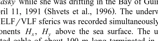
E of ELFu rVLF sferics was recorded simultaneously with two horizontal magnetic field components H , Hx y above the sea surface. The underwater electric antenna was an insulated cable of about 100 m long terminated in contact graphite electrodes. A side view of the antenna system alignment is shown in Fig. 1 and a top view is shown in Fig. 2. The cable antenna was hung up horizontally on floats at a depth of some 15 m and aligned along the water stream with respect to the vessel. The horizontal magnetic field components were received with two orthogonal air-core shielded coils, installed on the
Ž .
Ž .
Fig. 2. General alignment of the vessel and antenna system top view . Angles are measured clockwise from the North.
Ž
top deck being aligned lengthwise and crosswise to the vessel x and y coordinates
. 4
correspondingly . The r,w coordinate system of Fig. 2 is virtual. It is defined for every particular signal received by pivoting in the horizontal plane such that the r axis
Ž
is directed towards the source or in the opposite direction because of the sign ambiguity
. Ž
of the direction-finding procedure and w is perpendicular to r see Rafalsky et al.,
.
1995, and references therein .
Ž .
The signals of the three components underwater Eu and surface H , Hx y in the frequency range from 0.3 to 13 kHz were synchronously digitized with 12-bit analog-to-digital converters having a sampling rate of 100 kHz. Atmospheric waveforms of 40 ms long were captured with a digital buffer device and then, after visual selecting, were transferred to a computer for preliminary processing and storing on floppy disks. The
Ž .
details of measurements are described in Shvets et al. 1996 .
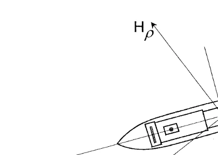
An example of a three-component atmospheric waveform recorded at 19:22:22 UT is
4
shown in Fig. 3. The pivoted coordinate system r,w is used. The vertical axes are
Ž .
graduated in arbitrary units H and H are graduated equally .r w
The initial high-frequency portion of the sferic is almost linearly polarized indicating only the H component, which is common for sferics and ensures a correctness of thew
direction finding procedure used. The ‘tail’ amplitude of both the magnetic components is the same indicating an almost circular polarization.
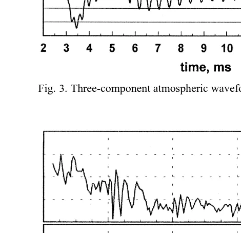
The spectra of the three field components of Fig. 3. are shown in Fig. 4. As the attenuation in the water grows with frequency, the higher frequencies in the Eu component are filtered out. Besides, E and H components indicate resonance maximau r
around 2 kHz, close to the first cut-off frequency of the Earth–ionosphere waveguide. A similar maximum in the H component is hidden because of strong interference betweenw
zero and first-order waveguide modes resulting in the oscillating pattern that can be seen in the spectrum from 2 kHz to 3.5 kHz. An analysis of such a pattern yields a rough
Ž .
Fig. 3. Three-component atmospheric waveform recorded at 19:22:22 UT.
3. Basic relationships
Let us imagine an oblique plane wave falling from air onto a homogeneous half-space
Ž 2 .
with refractive coefficient n n s´ at an angle of a as shown in Fig. 5. We consider
Ž .
two polarizations: parallel electric field lies in the incidence plane and perpendicular
Želectric field is perpendicular to the incidence plane ..
Let for the parallel polarization the H field component in the incident wave be:w
i
Hwsexp ik z cos
Ž
aqrsina.
.Then we can easily obtain for the field in the lower medium:
HwsT exp ik z5
Ž
Õqrsina.
, Ersh d0 5T exp ik z5Ž
Õqrsina.
Ž .
1Ž . Ž .
where: T5s 2 cos a rcos aqd5 —transmission coefficient for parallel polarization,
2
'
2 2d5sÕrn —normalized surface impedance for parallel polarization, Õs n ysina,
h0s
(
m0r´0 s120pV—characteristic impedance of free space. Similarly, for the perpendicular polarization we have:i
where: THs 2dH cos a r dH cos aq1 —transmission coefficient for perpendicu-lar poperpendicu-larization, d s1rÕ—normalized surface impedance for parallel polarization.
H
< <
We suppose that 1rn<cos a which is a common case for highly conducting
1
seawater. Then d fd f sd,Õfn, and T f2, Tf2d cos a.
H 5 n 5 5
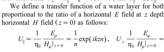
We define a transfer function of a water layer for both the basic polarizations to be proportional to the ratio of a horizontal E field at z depth to the corresponding surface
Ž .
horizontal H field zs0 as follows:
1 Er 1 1 Ew 1
U5s < s exp ikzn ,
Ž
.
UH < s exp ikznŽ
.
Ž .
3h0 Hw zs0 n h0 Hr zs0 n
Ž .
It should be noted that the transfer function definitions of Eq. 3 and hereafter are not conventional. They reflect the actual measurement configuration. The reason was
Ž . Ž .
that the one-component measurement of underwater electric field is natural because the long cable antenna always follows the water flow and an orthogonal component cannot be measured. Besides, the usage of two crossed magnetic antennas allowed us to analyze polarization.
Ž .
The transfer functions Eq. 3 for both polarizations are equal to each other and indicate no dependence on the incidence angle. The expected frequency dependence of the transfer function of a seawater layer of average salinity is given by:
'
1 z f
<U<; exp
ž
y/
Ž .
4250
'
ffor the both polarizations, where the frequency f is measured in Hertz and the z coordinate is measured in meters. Therefore we expected the experimentally obtained
Ž .
transfer function to be as simple and smooth function as Eq. 4 . The actual dependen-cies appeared quite different as we will see below.
4. Transfer functions obtained experimentally
Ž Ž . Ž ..
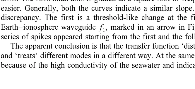
In Fig. 6 the theoretical Eqs. 3 and 4 and experimental frequency dependencies
Ž . Ž < .
of the transfer function Uws 1rh0 Eur Hw zs0 are shown being graded in arbitrary units. The horizontal axis is graded as a square root of frequency, making a comparison easier. Generally, both the curves indicate a similar slope. But there are two points of discrepancy. The first is a threshold-like change at the first cut-off frequency of the Earth–ionosphere waveguide f , marked in an arrow in Fig. 6. The second are regular1
series of spikes appeared starting from the first and the following cut-off frequencies. The apparent conclusion is that the transfer function ‘distinguishes’ waveguide modes
Ž .
and ‘treats’ different modes in a different way. At the same time, Eq. 3 are quite exact because of the high conductivity of the seawater and indicate no means for such a kind
of filtering. The way to resolve this contradiction is to take into account the initial polarization of the incident wave and an arbitrary arrival direction of the wave with regard to the linearly polarized underwater antenna.
In a general way, the E field component combines both polarizations:u
EusA E sinH w cqA E cos5 r c
s
Ž
AHcosasincqA cos5 c.
2dh0exp ik zŽ
Õqrsina.
sA
Ž
bcosasincqcosc.
2dh exp ik zŽ
Õqrsina.
Ž .
55 0
where A , A5 H being amplitudes of the waves of parallel and perpendicular polarization correspondingly, bsAHrA is the polarization factor of the incident wave.5
Similarly, we compose the H component wherej j is another arbitrary horizontal
Ž .
axis directed at an angle ofg to the r axis see Fig. 4b
HjsA H sin5 w gqA H cosH r g
s
Ž
A singyA cosacosg.
2 exp ik zŽ
Õqrsina.
5 H
sA sin
Ž
gybcosacosg.
2 exp ik zŽ
Õqrsina.
Ž .
65
We consider a more common transfer function 1 Eu bcosasincqcosc
Us s dexp ikzn
Ž
.
Ž .
7<
h0 Hj zs0 singybcosacosg
Ž .
Despite the transfer functions for both polarizations Eq. 3 are independent of the
Ž .
incidence anglea, the common transfer function Eq. 7 depends on a as well as on the
Ž .
polarization ratio b. Naturally, in the case of a pure polarization bs0 or bs` Eq.
Ž .7 does not depend on the incidence angle. Another case is when j is perpendicular to
Ž< < .
Now we can see that the transfer functions Eqs. 7 and 8 have the means to distinguish among different waveguide modes because each mode has its own incidence angle and polarization ratio.
5. Discussion and conclusions
Any mode of the Earth–ionosphere waveguide has its characteristic incidence angle on the boundaries of the guide. For a perfectly conducting model, which is useful for
Ž .
qualitative consideration, this angle for nth mode is Wait, 1962 : cosansnprkh, ns0,1, . . .
The angle an changes from zero at the corresponding cut-off frequency to almost
Ž .
At the frequencies lower than the first cut-off frequency f1 only one mode of zero order propagates. This mode is mostly vertically polarized so that the curve’s trend is
Ž .
close to the general law of Eq. 3 . The overall level of this part of the curve is dictated by the c angle.
Starting from f1 a couple of first-order modes appear being almost circularly
Ž .
polarized bf1 which results in the threshold-like change of Fig. 6. When further moving along the frequency axis the polarization ratio of the modes changes gradually, affecting the curve’s trend.
Each of the series of spikes mentioned above started from the cut-off frequency results from the oscillation patterns in spectrum of surface fields. A minimum in the field spectrum appears when two modes of the same amplitude but of opposite signs cancel each other. For the first series of spikes the modal sum is close to zero on the surface but it is not zero underwater because the water layer affects different modes differently. The opposite situation appears starting from f . The modes of the first and2
second order compensate each other underwater but they do not on the surface resulting in down-going spikes.
Eventually, we come to the following general conclusions.
Using a linearly-polarized underwater antenna makes the transfer function dependent on the incidence angle of the wave and its polarization as well as on the orientation of the receiving antenna
The water layer behaves as a spatial filter for modes in the Earth–ionosphere waveguide treating different modes in different ways. This makes the apparent transfer function strongly irregular.
Acknowledgements
This work was supported in part by Foundation of Fundamental Research under Ministry of Science and Technology of Ukraine, granta6.4r26.
References
Hayakawa, M., Ohta, K., Baba, K., 1994. Wave characteristics of tweek atmospherics deduced from direction finding measurement and theoretical interpretation. J. Geophys. Res. 99, 10733–10743.
Rafalsky, V.A., Nickolaenko, A.P., Shvets, A.V., Hayakawa, M., 1995. Location of lightning discharges from a single station. J. Geophys. Res. 100, 20829–20838.
Shvets, A.V., Lazebny, B.V., Kukushkin, A.S., 1996. Synchronous measurement of atmospherics on the sea surface and underwater. J. Atmos. Electr. 16, 221–226.