DEVELOPMENT OF GIS TOOL FOR THE SOLUTION OF MINIMUM SPANNING TREE
PROBLEM USING PRIM’S ALGORITHM
Suvajit Duttaa,*, Debasish Patraa, Hari Shankarb,*, Prabhakar Alok Vermab a Student, MCA, Narula Institute of Technology, Kolkata, West Bengal, 700109, India b Scientist, Geoinformatics Department, Indian Institute of Remote Sensing, Dehradun, 248001, India
KEY WORDS: Transportation Network, GIS Tool, Minimum Spanning Tree (MST), Prim’s Algorithm, Network Analysis
ABSTRACT:
A minimum spanning tree (MST) of a connected, undirected and weighted network is a tree of that network consisting of all its nodes and the sum of weights of all its edges is minimum among all such possible spanning trees of the same network. In this study, we have developed a new GIS tool using most commonly known rudimentary algorithm called Prim’s algorithm to construct the minimum spanning tree of a connected, undirected and weighted road network. This algorithm is based on the weight (adjacency) matrix of a weighted network and helps to solve complex network MST problem easily, efficiently and effectively. The selection of the appropriate algorithm is very essential otherwise it will be very hard to get an optimal result. In case of Road Transportation Network, it is very essential to find the optimal results by considering all the necessary points based on cost factor (time or distance). This paper is based on solving the Minimum Spanning Tree (MST) problem of a road network by finding it’s minimum span by considering all the important network junction point. GIS technology is usually used to solve the network related problems like the optimal path problem, travelling salesman problem, vehicle routing problems, location-allocation problems etc. Therefore, in this study we have developed a customized GIS tool using Python script in ArcGIS software for the solution of MST problem for a Road Transportation Network of Dehradun city by considering distance and time as the impedance (cost) factors. It has a number of advantages like the users do not need a greater knowledge of the subject as the tool is user-friendly and that allows to access information varied and adapted the needs of the users. This GIS tool for MST can be applied for a nationwide plan called Prime Minister Gram Sadak Yojana in India to provide optimal all weather road connectivity to unconnected villages (points). This tool is also useful for constructing highways or railways spanning several cities optimally or connecting all cities with minimum total road length.
1. INTRODUCTION
1.1 Background
In most scientific disciplines, software plays an important role for the solution of any transportation related problem like optimal routing, time analysis, services area analysis, closest facilities analysis (for emergency services), travelling sales man problem, vehicle routing problem, postman problem, supply-demand problem etc. A customized GIS tool helps users in their specific domain of work leads to the usage of recent software technologies according to their interest.
A graph (network) can be defined as G = G (E, V) where E is a set of edges and V is a set of vertices (nodes). A road transportation network is an interconnected linear system of nodes (junctions or vertices) and edges (lines or arcs) through which resources flow. Thus defined network can represent a vast structure while optimization problems are to be solved for chosen subsets of nodes only. Transportation is emerging as one of the biggest concerns for the people and congestion and lack of information cause delay in reaching destination. It is a demand of today that everyone wants to reach at the destination within a reasonable travel time or distance from the original place. In this study we are trying to find out the solution within these limits.
Geographic Information System (GIS) provides very useful tool for managing traffic related problems. Minimum Spanning Tree (MST) Problem is an optimization operation to connect each and every point (Network Junctions) with minimum distances or with minimum time period. There are a number of methods (algorithms) for the finding out a minimum spanning tree of a given road network. In this study we have applied rudimentary
algorithm called Prim’s algorithm for developing a customised GIS tool for the solution of minimum spanning tree problem.
Network analysis in GIS rests firmly on the theoretical foundation of the very famous branches of mathematic like graph theory and topology. Within graph-theory there are methods for describing, measuring and comparing graphs and techniques for proving the properties of individual graphs (networks) or classes of graphs. Some elements of graph theory are not concerned with the cartographic characteristics (e.g., shape or length) of the features that comprise a network but, rather, with the topological attributes of those features. The topological invariants of a network are those properties that are not altered by elastic deformations. Therefore, properties such as connectivity, adjacency and incidence are topological invariants of a network, since they will not vary if the network is deformed by a cartographic process, such as a projection. The permanence of these properties allows them to serve as a basis for describing, measuring, and analysing networks.
1.2 Minimum Spanning Tree (MST)
In graph theory, a tree can be defined as a connected graph G with n vertices and n-1 edges and does not having any sub-tour or loop among the vertices. A spanning tree of a graph (network) is a tree (sub-graph) consisting of all the nodes (vertices) of that graph. Thus a single graph (network) may consist of a number of spanning trees, in this case a graph also called the forest. And a minimum spanning tree (MST) of a network (graph) is a spanning tree (sub-graph) consisting of all the vertices of the same graph in such a way that the sum of weights of all edges is minimum among all such possible spanning trees of that network.
how unfavourable it is, and use this to assign a weight to a spanning tree by computing the sum of the weights of the edges in that spanning tree. A minimum spanning tree (MST) or minimum weight spanning tree is then a spanning tree with weight less than or equal to the weight of every other spanning tree (Figure 1).
Figure 1. Example of a MST of a given graph
Minimum-cost spanning trees are pervasive in many practical applications, few of them are -
1. The standard application of MST is in network design i.e. in telephone networks, TV cable network, computer network, road network, islands connection, pipeline network, electrical circuits, utility circuit printing, obtaining an independent set of circuit equations for an electrical network etc. to keep costs down.
2. The laying of communication links between any two stations involves a cost. The MST problem is to obtain a network of communication links which while preserving the connectivity between stations does it with minimum cost.
3. In the construction of highways or railroads spanning several cities, designing local access network, making electric wire connections on a control panel, laying pipelines connecting offshore drilling sites, refineries, and consumer markets minimum spanning tree technique is used. Like these, in many applications MST technique are widely used.
4. In the design of electronic circuitry, it is often necessary to make a set of pins electrically equivalent by wiring them together.
1.3 Mathematical Formulation of MST construction of weight matrix of the graph G is given by –
otherwise
The constraints of the formulation need to enforce that the edges in ET form a tree.
For example, the weight matrix of the graph G in Figure 2 is given below:
a) Graph G b) Weight Matrix of G c) MST of G
Figure 2. (a) Example of a graph G, (b) Weight Matrix (adjacency Matrix) of graph G, and (c) MST of graph G that: For example, Fig.2c shows the Minimum Spamming Tree T of the graph G (Fig. 2a) with a total cost of 56 obtained applying existing well known standard methods.
1.4: Prim’s Algorithm
Prim’s algorithm was developed by computer scientist Robert Prim in 1957. Prim’s Algorithm is a quick way of finding the Minimum Spanning Tree (or minimum connector) of a network (graph). This algorithm starts from an arbitrary node in the network, and builds upon a single partial minimum spanning tree, at each step adding an edge of lowest weight connecting the vertex nearest to but not already in the current partial minimum spanning tree with a condition that the properties of a tree should be maintained (connected sub-graph of n vertices and n-1 edges). It continues until the tree spans all the vertices in the given network. This algorithm is called greedy because at each step the partial spanning tree is augmented with an edge that is the smallest among all possible neighbouring edges.
Algorithm: Let a weighted, connected and undirected graph G = (E, V, W) where E, V and W are the sets of edges, vertices and edge weights respectively. Let U be the sub set of V and T be the required minimum spanning tree.
Where r is an arbitrarily chosen vertex from V
while U V do
Pick the edge i, j E of minimum weight
between U and V - U such that
i
U
and
j
V
U
j
U
U
;
)
j
,
i
(
T
T
end
The while loop is executed (n – 1) times, and finding an edge (each iteration) of minimum weight takes O(m) time, so yielding a total running time of O(mn). Each edge is added to the heap when one of its end points enters U, while the other is outside U. It is then removed from the heap when both its end points are in U. Adding an element to a heap takes O(logm) time, and deleting an element also takes O(logm) time. Thus, total running time in maintaining the heap is O(mlogm), which is O(mlog n) since m is O(n2). Thus, total running time in this heap implementation is O(mlog n). With Fibonacci heaps, Prim’s algorithm runs in O(m + n logn) time. This is the best known complexity for the problem.
The pseudo code of Prim’s algorithm using adjacency matrix in python script is shown in the Figure 3.
Figure 3. Pseudo Code of Prim's algorithm using Adjacency Matrix
1.4. Geographic Information System (GIS)
A geographic information system (GIS) is a computer-based tool for mapping and analysing geographic phenomenon that exist and events that occur, on Earth. GIS technology integrates common database operations such as spatial & non-spatial queries and spatial analysis with the unique visualization and geographic analysis benefits offered by maps. These abilities distinguish GIS from other information systems and make it valuable to a wide range of public and private enterprises for explaining events, predicting outcomes, and planning strategies. Map making and geographic analysis are not new, but a GIS performs these tasks
faster and with more sophistication than do traditional manual methods.
There is a common thinking of GIS as a single, well-defined, integrated computer system. However, this is not always the case. A GIS can be made up of a variety of software and hardware tools. The important factor is the level of integration of these tools to provide a smoothly operating, fully functional geographical data processing environment.
In graph theoretical terminology, a transportation network can be referred to as a valued graph, or alternatively a network. Directed links are referred to as arcs while undirected links as edges. Other useful terms with some intuitive interpretations are a path which is a sequence of distinct nodes connected in one direction by links; a cycle which is a path connected to itself at the ends; and a tree which is a network where every node is visited once and only once. The relationship between the nodes and the arcs, referred to as the network topology, can be specified by a node-arc incidence matrix: a table of binary or ternary variables stating the presence or absence of a relationship between network elements. The node-arc incidence matrix specifies the network topology and is useful for network processing.
1.5. GIS Customization
There are innumerable of Geographical Information System (GIS) software with plethora of capabilities, user with a specific problem needs specialized training to use the software. The role of customization is playing an important role in this scenario. If customized applications or tool with minimum number of menus/user interfaces are available it will help the user in better manner in solving their specific manner. Hence customize tools help non-technical users to utilize the functionalities of GIS without much technical expertise on that particular GIS software.
There are numerous tools available for GIS customization like Avenue, Arc Macro Language (AML), ArcObjects, VBA and COM, C# and .NET, Python, etc. AML was created by ESRI to unify application programming in ArcInfo across all platforms. It is a development environment that supports functions, variables, and basic programming constructions. However it lacks an integrated development environment with common control and access to the Windows application program interface (API), making the development of applications that are integrated with other desktop programs more challenging. Avenue is another object oriented environment to create customize environment in ArcView. ArcGIS is used to create customize GIS applications in Microsoft Visual Basic Environment (VBE) using COM model. In light of ESRI’s plan to phase out Visual Basic for Applications (VBA) in their ArcGIS products, customization of GIS tasks have started being done extensively with Python.
1.6. Python and GIS
applications is also easily supported. Python provides a complete set of tools for any GIS toolbox and more options are available in combination with ArcGIS.
The simple syntax of Python certainly helps researchers who want to construct environmental models, because it results in a language that is easy-to-learn for people without special knowledge of programming. Another advantage of Python is that it completely hides technical details with which users of systems programming languages need to concern themselves.
The main objectives of this study are i) to create the digital database consisting of roads and junctions feature classes in GIS environment and assigning attribute information to all the features for performing the solution of MST, ii) Development of GIS tool for the solution of MST using Prim’s Algorithm in Python Shell, iii) Linking of digital database with MST tool and performing the solution. In addition to the above main objectives there are few sub-objectives in this study like Collection of field data, Spatial & non-spatial data entry and editing, creation of network topology and network dataset and development of script using python language.
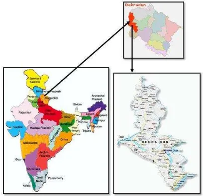
2. STUDY AREA
The study area for this study has chosen the Dehradun, a capital city of Uttarakhand state of India as shown in Figure 4. It lies between the parallel 30° 17’35’’N to 30° 18’ 18’’ N and meridian 78°03’00’’E to 78°03’41’’E which covers an area of approximately 3 Sq.Km. Broadly speaking, study area is locating to the Nehru colony covering the region Dharampur chowk to Defense colony along the National Highway 7. A dry river by named Rispana is situated next to defense colony is also considered as part of this project. The study area mainly covers in respect of Dehradun district of Uttrakhand, India.
Figure 4. Study Area (Dehradun)
3. LITERATURE REVIEW
The construction of MST of an undirected connected weighted road network belongs to the group of classical combinatorial optimization problems, which can be solved by greedy heuristics in polynomial time (Graham, 1985). Boruvka have first identified practical problem related to Minimum Spanning Tree in 1926. Recently, a number of practically relevant variants of MST problem have been studied. For example the Degree-Constrained MST problem (Pagacz, 2006), Bounded Diameter MST problem formulated by Nghia and Binh (Nghia, 2008), and the Capacitated Minimum Spanning Tree problem (Jothi, 2005 and Zhou, 2006). Many computationally efficient algorithms have been developed by many researchers (Gen M, 2000, Oncan, 2007, Salazar-Neumann, 2007 and Zhou, 1998) for the solution of deterministic MST problem. Kruskal’s algorithm and Prim’s algorithms are the two most commonly used for constructing MST of a graph.
Giri Narasimhan et al. (2001) gave a practical algorithm that solves the generalized MST problem. They prove that for uniformly distributed points, in fixed dimensions, an expected (n log n) steps suffices to compute the generalized MST using well separated pair decomposition. Their algorithm, GeoMST2, mimics Kruskal's algorithm (J.B. Kruskal, 1956) on well separated pairs and eliminates the need to compute bichromatic closest pairs for many well separated pairs.
J. J. Brennan (1982) presented a modification to Kruskal's classic minimum spanning tree (MST) algorithm (J.B. Kruskal, 1956) that operated similar in a manner to quicksort; splitting an edge set into ‘light’ and ‘heavy’ subsets. Recently, Osipov (Vitaly, 2009) further expanded this idea by adding a multi-core friendly filtering step designed to eliminate edges that were obviously not in the MST (Filter-Kruskal). Currently, this algorithm seems to be the most practical algorithm for computing MSTs on multi-core machines.
In 2008, Derek Karssenberg et al. has developed a new tool that allows scientists and engineers without specialist knowledge in programming convert theories to computer models simulating landscape change through time. The tool was developed in python and was called PC-Raster and its main strengths were its extendibility and scalability. It was also observe that python provided language features that are very useful to construct large models while keeping the readable.
In 2011, Thomas R. Etherington has developed a series of python script based on GIS tools for using landscape genetic studies. The script generated was used to convert files, visualize genetic relatedness and measure landscape connectivity. The scripts were housed in an Arc Toolbox and hence provided easy access to researchers to provide the option of further development by the user community, and reduce the amount of time that would be spent developing common solutions.
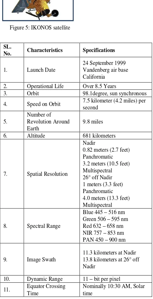
Figure 5: IKONOS satellite Technically speaking, geoprocessing tools are functions available
from ArcPy—that is, they are accessed like any other Python function. However, to avoid confusion, a distinction is always made between tool and nontool functions (such as utility functions like ListFeatureClasses).
Tools are documented differently than functions. Every tool has its own tool reference page in the ArcGIS Desktop help system. Functions are documented in the ArcPy documentation. Tools return a result object; functions do not.
Tools produce messages, accessed through a variety of functions such as GetMessages(). Functions do not produce messages. Tools are licensed by product level (ArcView, ArcEditor, or ArcInfo) and by extension (Network Analyst, Spatial Analyst, and so on). You can find what license levels are required on the tool's reference page. Functions are not licensed—they are installed with ArcPy.
A tool performs a small, essential operation on GIS data. There are four types of tools, as shown in the table below. All tools, regardless of their type, work the same way; you can open their dialog box, you can use them in Model Builder, and you can call them from software programs.
Table 1. ArcGIS Tools
4. MATERIAL AND METHOD
4.1 Data Used
4.1.1 Description of the Satellite Image
Mainly two types of data have been used in this project:
IKONOS high resolution imaginary of Nehru colony Field Data
IKONOS Satellite System
The IKONOS Satellite (Figure 5) is a high spatial resolution (4.0 meter multispectral) satellite operated by Geo Eye. Its application include both urban and rural mapping of natural resources and of natural disasters, tax mapping, agriculture and forestry analysis, mining, engineering, construction and change detection. Its high
resolution data makes an integral contribution to homeland security, costal monitoring and facilities 3D Terrain analysis.
The Sensor Characteristics for
2. Operational Life Over 8.5 Years
3. Orbit 98.1degree, sun synchronous
4. Speed on Orbit 7.5 kilometer (4.2 miles) per
6. Altitude 681 kilometers
7. Spatial Resolution ArcObjects and a compiled programming language like .NET.
Model tool. These tools are created using ModelBuilder.
Script tool. These tools are created using the Script tool wizard and run a script file on disk, such as a Python file (.py), AML file (.aml), or executable (.exe or .bat).
Perform the Transportation Network Analysis Using the
GIS Tool
Result & Analysis Conclusion Georeferenced IKONOS
satellite data (WGS_1984, UTM, 44N)
Prepare python script for MST Problem using
Prim’s Algorithm
Database Creation
Satellite Data
Digitization of Satellite Data (in
ArcGIS)
Field Dataset
Feature Class:
Major_Roads
Minor_Roads
Network Dataset Creation & Editing Spatial Data Entry &
Editing
Topology Creation & Validation Attribute Data Entry
Link The MST tool with the necessary input data
Create a feature layer of the resultant outcome of
MST Script Find out the MST on the
geodatabase Use geodatabase data in
the MST Python script Use ArcPy Data access module for accessing
geodatabase
Modify the script by setting parameters
functions
Add an ArcGIS Toolbox
Add the script tool into Toolbox setup the necessary
Google Earth. Basically we have taken the information about the road conditions, speed limits, traffic conditions, and road types.
4.1.2 Transportation Network
In Dehradun transport network is basically based on railway network and road network as shown in Figure 6. All major cities are connected with Dehradun through railway network. Road connectivity is also good with Uttar Pradesh, Delhi, Punjab and Haryana. In our study we are considering Major, Minor roads and streets of the road network. Two features classes have 41 rows, 9 columns and 183 rows, 9 columns respectively.
Figure 6. Road Network of Nehru Colony, Dehradun
4.2 Software Used
In this study we have used ESRI desktop product ArcGIS 10.0 software for creation of GIS digital geodatabase, topology creation, network dataset creation.
We have used Python 2.6, Eclipse (Keplar) and ArcPy site-package of ArcGIS 10.0 for ArcGIS tool development. MS office 2007 is used for report writing and power point presentation.
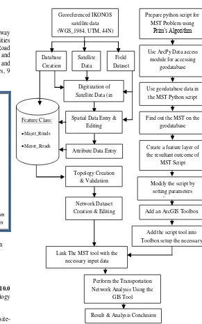
4.3 Methodology
The methodology under this study is summarized in two sections,
1. Database Creation 2. Tool Development
4.3.1 Flow Chart
Figure 7. Flow chart of methodology
The first section in Figure 7 is about selecting the area which requires high resolution satellite imaginary of the selected study area. Next step is to Geo-referencing the high resolution satellite image and setting the datum as WGS 1984 and projection as UTM 44N followed by digitizing the road network. After digitization assign the attribute data to the Roads by creating a Geodatabase, Feature Database and Feature Classes.
script with ArcGIS interface. Through ArcPy we connect the Geo-database with python script and modified the script according to the ArcGIS tool creation process.
4.3.2 Database Creation
To create the geodatabase the first think needed is a satellite image of our proposed study area. In this study we have selected IKONOS satellite image of the study area as the reference layer for preparing the geodatabase. The coordinate system of image is WGS 84 UTM zone 44N. Then have created the geodatabase by digitizing roads (Line Feature class) all the necessary roads. The road feature class basically divided into three category Major_Roads, Minor_Roads and Streets. The collected field data is also added to the database like particular speed limit of the road, road condition, Road type and capacity as well.
4.3.3 Spatial and Non-spatial Data Entry and Editing
We have entered spatial data (road features) by means of digitization of all road features in the geodatabase. In non-spatial data entry we have added all necessary attribute fields required to solve MST problem as shown in Table 3. Between those attributes three attributes (OBJECTID, Shape and SHAPE_Length) are being automatically filled by ArcGIS 10.0 itself and rest of the fields are filled as per the requirement of MST.
Sl.
Table 3. Attribute of Line Features
For line feature we have used SHAPE_Length and Time as the impedance (cost factor) of the corresponding line feature. In our MST algorithm we need prefix and suffix as the vertices and SHAPE_Length and Time as cost function. The time is calculated as the travelling time with the help of maximum allow speed mistakes in the digitization and attributes, these mistakes we have corrected (edited) using ArcGIS software’s Edit Tools. After editing all the features using edit tool, there are further chances of errors in the database (overlapping or intersection among the features). Further, these types of errors were eliminated by the creation of topological rules under topology creation of the geodatabase.
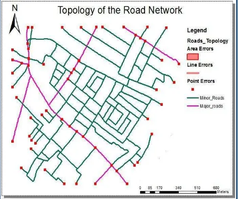
4.3.4 Creation and validation Network Topology
After spatial data entry and editing there may be some chances of error can be occurred respect to connectivity and continuity (Figure 8). To handle these problems we have created the topology of feature class dataset which includes all the line features mentioned above .
Figure 8. Topology for the Road Network
In topology creation part, the following topology rules have been created by keeping 0.10 meters of cluster tolerance:
1. Major_Roads must not overlap
2. Major_Roads must not overlap with Minor_Roads 3. Minor_Roads must not overlap
4. Minor_Roads must not overlap with Major_Roads 5. Major_Roads must not have dangles
6. Minor_Roads must not have dangles
4.3.5. Network Dataset Creation
Figure 10. Adding a Script Tool Turns: Global turns, 3) Attributes: Travel Time (cost type), Travel
Distance (cost type), Oneway (restriction type).
Figure 9. Network Dataset
4.3.6 ArcGIS script tool development
ArcGIS scripting provides flexibility to the software, user can make his personal customized script tool for data analysis in the ArcGIS as the way he likes. In this study we have made our own customized tool to solve MST problem using the Prim’s algorithm. For the development of our MST script tool we have followed few simple steps:
At first we have implement the Prim’s algorithm in python using the adjacency matrix process. To make the python script Eclipse IDE and Python 2.6 are being used, program is experimented over a small graph and the outcome gives the minimum spanning tree and minimum cost of that graph considering all Vertices.
ArcGIS 10.0 introduces ArcPy, a Python site package that encompasses and further enhances the ArcGIS scripting module introduced at ArcGIS 9.2 as shown in Figure 10. ArcPy provides a rich and dynamic environment for developing Python scripts while offering code completion and integrated documentation for each function, module, and class. In second step we use ArcPy data access modules for accessing geodatabase. From database we have read network dataset, major_roads and minor_roads feature classes. From the feature classes of the geodatabase attribute PREFFIX, SUFFIX have been taken as starting vertex and end vertex, between SHAPE_Length and Time we have selected SHAPE_Length as cost factor adjacency matrix have been made as the input of Prim’s algorithm, as output we have got the minimum cost of the road network considering all the Network Junctions.
A layer file (.lyr) is being created (Figure 11) by using ArcPy Feature Layer Management Tool to display the resultant minimum spanning tree data (Minimum SHAPE_Lengths) on the ArcMap screen and to save the result as a layer.
Next step is to modify the script tool by setting up the parameter functions and index values, so that user can take input directly from the ArcGIS window. An ArcGIS toolbox has been created and the script then added into it by setting up all the input and output parameters. Parameters in the ArcGIS script tool are the options of giving input and taking output from the python script. After finalizing the process of adding script tool we can run the tool in the ArcMap by taking necessary inputs from the user “Figure 12”.
Figure 12. User interface of the MST tool considering all necessary inputs
5. RESULTS AND DISCUSSIONS
For testing of the tool we have run the Network Analysis Tool (Minimum Spanning Tree Layer) on our created geodatabase. From Network Dataset we have taken Major_Roads and Minor_Roads feature classes, and Prefix and Suffix attributes have been taken as the edges and SHAPE_Length cost as the input for the MST Tool. The output of MST is shown in Figure 13.
Figure 13. Minimum Spanning Tree of the road network considering all road
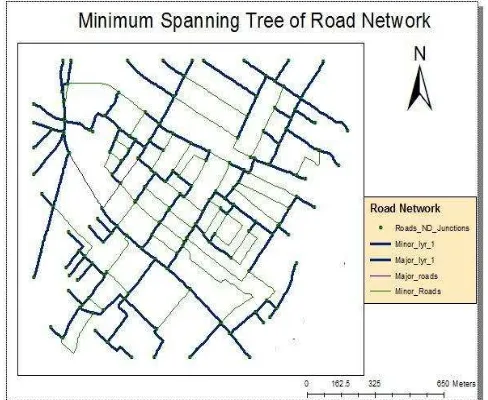
The following “Figure 14” shows the output of MST Tool using all the necessary parameters. As we can see every network junctions are being visited, thus the MST tool gives a proper minimum spanning tree of the road network.
Figure 14. Minimum Spanning Tree of Road Network considering all the network junctions
When the processing is being done we get the output as a Minimum Spanning Tree layer of the Road Network. The output gives a successful Minimum Spanning Tree of the road network, as the result shown in figure 16 every Network Junctions (Vertex) is being visited. Figure 15 shows the results, minimum cost of the road network (14264.8058004644 meters) and all the necessary inputs and outputs of the tools.
We have tested the tool with different starting point, but every time it gives us the same result as the following output.
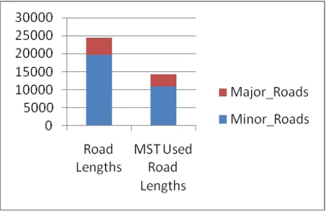
The MST Tool is being tested over the Geodatabase of Nehru Colony of the Dehradun City of Uttrakhand, which contains Minor_Roads total length 19699.995002 meters and Major_Roads total length 4817.49043 meters containing 168 network junctions. After running the MST Tool we can clearly calculate that to cover all 168 network junctions the minimum length of Minor_Roads have to cover is 10887.118224 meters and length of Major_Roads to cover is 3377.687577 meters. Out of 183 Minor_Roads and 41 Major_Roads only 132 Minor_Roads and 35 Major_Roads are used to cover all 168 network junctions and give the solution to Minimum Spanning Tree problem. Figure 16 shows the amount of used roads by a bar chart representation.
Figure 16. Bar chart of Road Lengths
6. CONCLUSIONS
The paper presented a GIS based tool with new simple and efficient technique to find and construct MST of an undirected connected weighted road network. As there are several applications of Minimum Spanning Tree (MST), this GIS tool will be useful to solve such related problems.
The Minimum Spanning Tree (MST) tool executed using the data of Nehru colony, Dharampur Road, Dehradun. In the implementation of GIS tool for Minimum Spanning Tree problem is used in GIS environment.. The conclusion towards this study is that we have tested the implementation of python script and this GIS tool by python scripting worked correctly for the given inputs. From the analysis, it can be concluded that Prim’s algorithm for Minimum Spanning Tree problem which works in background give the best result to minimize the total travel distance and total travel time over a road network.
This paper strives to demonstrate a practical MST algorithm that is theoretically efficient on geographically distributed point sets. To that effect we introduced the Prim’s algorithm, an efficient, parallelizable MST algorithm that in both theory and practice accomplished our goals. The results obtained by this GIS tool are having greater satisfaction in order to minimize the total road length which is the essential requirement for connecting major nodes (junctions) with each other.
RECOMMENDATIONS
Network analysis in GIS provides solution to Minimum Spanning Tree problem for find out the minimum span of the road network. It is recommended as per the study carried out that GIS is an effective tool to search and select most suitable route for the optimum transportation cost with minimum travel distance and minimum travel time. This MST tool can be applied for a nationwide plan called Prime Minister Gram Sadak Yojana in India to provide optimal all weather road connectivity to unconnected villages. This tool is also useful for constructing highways or railways spanning several cities optimally or connecting all cities with minimum total road length. This tool can also be used to lay out electrical networks in order to minimize the total length of wire in the houses.
Graham, R.L., Hell, Pavol, On the history of the minimum spanning tree problem. Annals of the History of Computing. 7 (1), 44–57, 1985.
Pagacz, Anna, Raidl, Gunther, Zawislak, Stanisaw, Evolutionary approach to constrained minimum spanning tree problem – commercial software based application. Evolutionary Computation and Global Optimization, 331–341, 2006.
Nghia, Nguyen Duc, Binh, Huynh Thi Thanh, Heuristic algorithms for solving bounded diameter minimum spanning tree problem and its application to genetic algorithm development, advances in greedy algorithms. Witold Bednorz, 2008.
Jothi, Raja, Raghavachari, Balaji, Approximation algorithms for the capacitated minimum spanning tree problem and its variants in network design. ACM Transactions on Algorithms 1 (2), 265–282, 2005.
Zhou, Gengui, Cao, Zhenyu, Cao, Jian, Meng, Zhiqing, A genetic algorithm approach on capacitated minimum spanning tree problem. International Conference on Computational Intelligence and Security, 215–218, 2006.
Gen M, Cheng R, Genetic Algorithms and Engineering Optimization, John Wiley, New York, 2000.
Oncan T, Design of capacitated minimum spanning tree with uncertain cost and demand parameters, Information Sciences, 177(20), 4354-4367, 2007.
Salazar-Neumann M, The robust minimum spanning tree problem: Compact and convex uncertainty, Operations Research Letters, 35(1), 17-22, 2007.
Zhou G, Gen M, An effective genetic algorithm approach to the quadratic minimum spanning tree problem, Computers and Operations Research, 25, 229-247, 1998.
Y. Xu, V. Olman, and D. Xu. Clustering gene expression data using a graph-theoretic approach: An application of minimum spanning trees. Bioinformatics, 18, 536–545, 2002.
Giri Narasimhan and Martin Zachariasen. Geometric minimum spanning trees via well-separated pair decompositions. J. Exp. Algorithmics, 6:6, 2001.
J.B. Kruskal. On the shortest spanning subtree of a graph and the traveling salesman problem. In Proc. American Math. Society, pages 7- 48, 1956.
J.J. Brennan. Minimal spanning trees and partial sorting. Operations Research Letters, 1(3):138-141, 1982.
Vitaly Osipov, Peter Sanders, and Johannes Singler. The Filter-kruskal minimum spanning tree algorithm. In Irene Finocchi and John Hershberger, editors, ALENEX, pages 52-61. SIAM, 2009.