STUDY ON IMPROVEMENT OF ACCURACY IN INERTIAL PHOTOGRAMMETRY BY
COMBINING IMAGES WITH INERTIAL MEASUREMENT UNIT
Hideaki Kawasakia, Shojiro Anzaib, and Toshio Koizumic
a Tokyo Metropolitan Government Bureau of Port and Harbor. [email protected] b Asia Air Survey. [email protected]
c Professor of Department of Architecture and Civil Engineering, Chiba Institute of Technology. [email protected]
Commission V, WG V/3
KEY WORDS: IMU(Inertial Measurement Unit), Inertial photogrammetry, Photogrammetry, Terrestrial photogrammetry, SfM(Structure from Motion)
ABSTRACT:
Inertial photogrammetry is defined as photogrammetry that involves using a camera on which an inertial measurement unit (IMU) is mounted. In inertial photogrammetry, the position and inclination of a shooting camera are calculated using the IMU. An IMU is characterized by error growth caused by time accumulation because acceleration is integrated with respect to time.
This study examines the procedure to estimate the position of the camera accurately while shooting using the IMU and the structure from motion (SfM) technology, which is applied in many fields, such as computer vision.
When neither the coordinates of the position of the camera nor those of feature points are known, SfM provides a similar positional relationship between the position of the camera and feature points. Therefore, the actual length of positional coordinates is not determined. If the actual length of the position of the camera is unknown, the camera acceleration is obtained by calculating the second order differential of the position of the camera, with respect to the shooting time. The authors had determined the actual length by assigning the position of IMU to the SfM-calculated position. Hence, accuracy decreased because of the error growth, which was the characteristic feature of IMU. In order to solve this problem, a new calculation method was proposed. Using this method, the difference between the IMU-calculated acceleration and the camera-calculated acceleration can be obtained using the method of least squares, and the magnification required for calculating the actual dimension from the position of the camera can be obtained. The actual length can be calculated by multiplying all the SfM point groups by the obtained magnification factor. This calculation method suppresses the error growth, which is due to the time accumulation in IMU, and improves the accuracy of inertial photogrammetry.
1. INTRODUCTION
In inertial photogrammetry, the position and inclination of a shooting camera are calculated using the IMU. An IMU is characterized by error growth caused by time accumulation because acceleration is integrated with respect to time.
This study examines the procedure to estimate the position of the camera accurately while shooting using the IMU and the structure from motion (SfM) technology, which is applied in many fields, such as computer vision.
2. THEORY OF INERTIAL PHOTOGRAMMETRY PROPOSED IN THIS PAPER
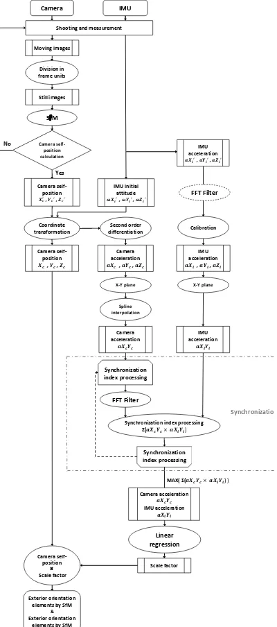
The inertial photogrammetry proposed in this paper is based on the theory of giving a scale to SfM data. Figure 1 shows the analysis flow of the inertial photogrammetry proposed here.
2.1 Shooting and Measuring
Firstly, moving images must be shot with the camera, and acceleration must be measured with the IMU. Once shot, the moving images must be written as still images in units of frames. The written images must be analyzed by the SfM in order to obtain the relative object three-dimensional point group data, the camera position and inclination data.
2.2 Exterior Orientation Elements of Camera by SfM
SfM estimates the relative position and inclination of the shooting camera according to the position relationship of the
feature points that are commonly recorded on multiple images, and calculates the three-dimensional coordinates of the feature points.
Equation (1) is the perspective transformation equation that represents the relationship between the image-recorded two-dimensional points (left-hand side) and the actual three-dimensional points (right-hand side). The 3 × 3 matrix in equation (1) that contains focal length f represents the interior orientation elements (lens distortion, principal point position, etc.) of the camera. The parameters of the matrix are determined by calibrating the camera. The 3x4 matrix that contains camera position t and inclination r represents the exterior orientation elements of the camera. In the camera position analysis by SfM, the initial position of the camera is used as the origin and the initial attitude of the IMU is used as the attitude of the camera.
[ ] = [� ��� � ] [ ] [ ] (1)
:Scale factor
, :Two-dimensional coordinates of image
� : Focal length
, :Size of imaging device
, :Center position of image
��: Inclination of u-axis and v-axis
~ :Inclinations of camera
, , :Position of camera
, , :Three-dimensional coordinates of camera
2.3 Extraction of Acceleration from SfM data
When the SfM analysis is performed without giving the initial coordinates, a model that is in similar positional relationship with the true model is generated. This is because the scale factor s is not determined for the obtained camera exterior orientation elements or for the three-dimensional point group data. Next, the IMU acceleration data is used to assign a scale to the calculated camera position. However, if the IMU acceleration is integrated, error growth occurs through time. To solve this problem, we perform second-order differentiation of the SfM-obtained camera position with respect to time, instead of integrating the IMU acceleration. In this paper, the camera acceleration is defined as the value obtained by performing second-order differentiation of the camera position by time. The shot frame rate (fps) is used as the time for the differentiation.
The scale factor is obtained by comparing the camera acceleration with the IMU acceleration. This provides an assigned scale to the SfM data without having to perform integration.
Fig. 1 Analysis flow used in this paper
3. EXPERIMENT
3.1. Purpose of Experiment
The purpose of this experiment is to validate the new technique (hereinafter also referred to as this technique) that calculates a scale by using the camera acceleration and IMU acceleration.
This experiment also validates a synchronization method that does not require hardware-based synchronizers.
3.2. Experimental Location and Method
The camera used in this experiment is a SONY α7S (Figure 2) and the IMU unit is a Seiko Epson M-G350/S4E5A0A0A1 (Figure 3). This experiment also uses a Gimbal Stabilizer DJI RONIN-M (Figure 4) to suppress the effects of camera shake on moving images during shooting.
The experimental site is located to the south of the No. 2 building of the Chiba Institute of Technology (Figure 5). The experimental method is shown in Figure 6.
The experiment was performed using single-axis walking movement from the 0-meter origin to the 60-meter location (Figure 6). The coordinates used in this experiment are shown in Figure 6. The camera was fixed on a moving hand-held gimbal stabilizer. Firstly, keeping the camera horizontal by using the gimbal stabilizer, the IMU operation was started, and walking was halted for 10 seconds. Next, moving-image shooting by the camera was started, and walking was halted for a further 3 seconds. The hand-held gimbal stabilizer was then walked forward in a straight line, with the camera shooting in the same direction. The walking speed was accelerated and then decelerated every 10 meters. After reaching the 60-meter point, walking was halted for 3 seconds and the camera shooting was then terminated, followed 10 seconds later by termination of the IMU measurement.
Accuracy is validated by two tests. The first test uses this technique and compares the camera exterior orientation elements (which are obtained by the IMU alone) with the true values. The true values are the camera exterior orientation elements that are calculated by the photogrammetry using reference (i.e., given) points. The second test uses this technique and compares the three-dimensional distances of the reference points (which are calculated by conventional inertial photogrammetry; see Figure 6) with the true values. The three-dimensional distances are the straight-line distances up to the targets in the three-axis coordinates. The true values of the reference points are measured by using the total station.
Fig. 2 Camera SONY α7S
Fig. 3 IMU Seiko Epson M-G350/S4E5A0A0A1
Synchronization
Fig. 4 Gimbal stabilizer DJI RONIN-M
Fig. 5 West passage of No. 1 building of Chiba Institute of Technology
Fig. 6 Experimental method
3.3. Experimental Results
3.3.1. Camera Acceleration and IMU Acceleration
Figures 7, 8, and 9 show the camera accelerations calculated by second-order differentiation and the camera distances obtained by SfM.
As shown in Figure 7, the camera is accelerated and decelerated on the X-axis at regular intervals. This means that the locus obtained by performing acceleration and deceleration every 10 meters is reflected in this graph. However, in Figure 7, the camera distance on the X-axis is approximately 38 meters when the movement distance is 60 meters. This is because the scale is not determined in this case.
Figures 10, 11, and 12 show the IMU accelerations (calculated by the IMU) and the IMU distances obtained by
second-order integration. As shown in Figure 10, the IMU is accelerated and decelerated on the X-axis at regular intervals in a similar way to the camera acceleration and deceleration shown in Figure 7. In Figures 11 and 12, the IMU accelerations are seen to be larger than the camera accelerations shown in Figures 8 and 9. This is because the IMU detects vibrations due to walking. In Figures 10 and 11, the IMU distances increase with respect to time because second-order integration is performed.
If the scale factor is calculated from the camera position and IMU position, the IMU acceleration is integrated; therefore, the above errors increase. To solve this problem, second-order differentiation of the camera position obtained by SfM should be performed, and the scale factor should be determined from the camera acceleration and the IMU acceleration.
Fig. 7 X-axis acceleration and position of camera
Fig. 8 Y-axis acceleration and position of camera
Fig. 9 Z-axis acceleration and position of camera
Fig. 10 X-axis acceleration and position of IMU
○ ○ ○ ○ ○ ○
Fig. 11 Y-axis acceleration and position of IMU
Fig. 12 Z-axis acceleration and position of IMU
As the camera that was actually used is not synchronized with the IMU through a hardware-based synchronizer, the camera must be synchronized with the IMU in another way. We achieved this synchronization instead by calculation. The rotation angle of the IMU can be obtained by integrating the angular velocity. As shown in Equation (2), the acceleration on the plane is calculated from the X-axis acceleration and Y-axis acceleration.
� �= √ � + � (2)
: Acceleration in shooting direction
: Acceleration in the direction perpendicular to shooting direction
� � : Distance of the plane direction
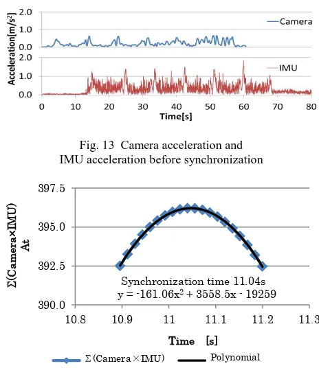
Figure 13 shows the camera and IMU accelerations on the plane. Each unit is started at time t = 0. The same synchronization method is used as in the isoperimetric problem for calculating the maximum area of a figure. When it can be assumed that the camera and IMU accelerations are equal, the maximum value of the product indicates the position in which the camera and IMU accelerations coincide. Therefore, the synchronizing position is obtained when the product of the
� �: Plane vector of IMU acceleration
� �: Plane vector of camera acceleration
T: Time n: Number of data
Figure 14 shows the graph of the area At (obtained by Equation 3) and the polynomial using the area At. A more precise synchronizing position is obtained by using this polynomial.
Figure 15 shows the synchronization result obtained by this technique. When the camera acceleration is compared with the IMU acceleration, as shown in Figure 15, the acceleration generated in the experiment occurs at about the same time as that indicated with green lines. This means that synchronization can be performed by this technique.
Fig. 13 Camera acceleration and IMU acceleration before synchronization
Fig. 14 Synchronizing time of camera and IMU
Fig. 15 Camera acceleration and IMU acceleration after synchronization
3.3.2. Calculation of Scale Factor
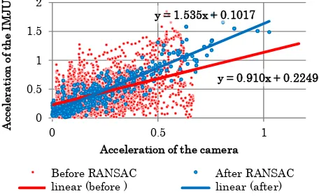
Figure 16 shows the camera-IMU correlation diagram, in which outliers are excluded by the RANSAC processing. The red points in this figure indicate the correlation of the camera and IMU before outliers are excluded by RANSAC. The red line indicates the linear regression obtained with the red points. The blue points are the points obtained by RANSAC. The blue line indicates the linear regression obtained using RANSAC.
The scale factor is required to make the camera acceleration the same as the IMU acceleration. The scale factor can be obtained by Equation (4):
-200
Σ(Camera×IMU) Polynomial The International Archives of the Photogrammetry, Remote Sensing and Spatial Information Sciences, Volume XLI-B5, 2016
= + � = (4)
: Acceleration of IMU : Acceleration of camera s : Scale factor
a,b : Constant terms
When Equation (4) is used, the scale factor used in this experiment is 1.535. The actual scale can be calculated by multiplying the SfM-calculated camera position and the object three-dimensional position by this scale factor.
Fig. 16 Correlation diagram after RANSAC processing
3.3.3. Validation of Theory and Accuracy
Figure 17 shows the comparison of three-dimensional distances of the camera exterior orientation elements obtained by this technique (a combination of SfM with IMU) and those obtained by the conventional technique using the IMU alone (simple integration). These distances are compared with the true values, which are the photogrammetry values obtained using the reference points. As shown in this figure, when the conventional technique using the IMU alone is applied, error growth can be observed in the IMU position due to integration with time. On the other hand, when this new technique is applied, the IMU acceleration is not integrated but is used instead only for scale-factor calculation. This prevents error growth due to integration from occurring, and suppresses accuracy reduction through time.
Figure 18 shows the comparison of three-dimensional distances of the validated points obtained by this new technique (a combination of SfM with IMU), the conventional technique using the IMU alone (simple integration), and the ground photogrammetry using reference points. These distances are compared with the true values. As shown in Figure 18, when the errors generated by this new technique are compared with those generated by the conventional technique using the IMU alone, it can be confirmed that the measurement accuracy is improved by correctly estimating the exterior orientation elements of the camera.
Instead of integrating the IMU acceleration to obtain the exterior orientation elements, the IMU acceleration can be used instead to assign the scale to the camera position obtained by SfM. This reduces the disadvantage of inertial photogrammetry, in that it suppresses error growth due to IMU integration occurring over time.
Fig. 17 Accuracy comparison using exterior orientation elements of the camera
Fig. 18 Accuracy comparison using validated points
4. CONCLUSIONS
1. We devised and validated an SfM scale assignment technique using IMU acceleration and second-order differentiation of camera position. (SFfAM:Scale Filter from Acceleration Method)
2. We validated the effect of the camera-IMU synchronization obtained by calculation when the camera is not connected to the IMU through a hardware-based synchronizer.
3. This technique also helps to improve the positioning accuracy in the inertial survey using the IMU.
y = 0.910x + 0.2249
Acceleration of the camera
RANSAC前 RANSAC後