SPCA ASSISTED CORRELATION CLUSTERING OF HYPERSPECTRAL IMAGERY
A. Mehta a,*, O. Dikshit a
a
Department of Civil Engineering
Indian Institute of Technology Kanpur, Kanpur – 208016, Uttar Pradesh, India [email protected], [email protected]
KEY WORDS: Hyperspectral Imagery, Correlation Clustering, ORCLUS, PCA, Segmented PCA
ABSTRACT:
In this study, correlation clustering is introduced to hyperspectral imagery for unsupervised classification. The main advantage of correlation clustering lies in its ability to simultaneously perform feature reduction and clustering. This algorithm also allows selection of different sets of features for different clusters. This framework provides an effective way to address the issues associated with the high dimensionality of the data. ORCLUS, a correlation clustering algorithm, is implemented and enhanced by making use of segmented principal component analysis (SPCA) instead of principal component analysis (PCA). Further, original implementation of ORCLUS makes use of eigenvectors corresponding to smallest eigenvalues whereas in this study eigenvectors corresponding to maximum eigenvalues are used, as traditionally done when PCA is used as feature reduction tool. Experiments are conducted on three real hyperspectral images. Preliminary analysis of algorithms on real hyperspectral imagery shows ORCLUS is able to produce acceptable results.
* Corresponding author.
1. INTRODUCTION
In recent years, hyperspectral imaging has become an important tool for information extraction, especially in the remote sensing community (Villa et al., 2013). Hyperspectral imagery contains hundreds of narrow spectral bands which are continuous and regularly spaced in the visible and infrared region of electromagnetic spectrum. Thus, due to their high spectral resolution, hyperspectral imagery, as compared to multispectral imagery, provides an opportunity for more precise information extraction. Widely used technique for information extraction, from hyperspectral imagery is classification. Two main schemes for classification are supervised and unsupervised classification (or clustering). Supervised classification methods make use of training data whereas clustering method does not require the same. Although generally supervised classification methods are more successful in providing higher classification accuracy as compared to unsupervised methods (Paoli et al., 2009), in reality, collection of high quality training sample is very expensive and time consuming procedure. As a result, availability of quality training sample is limited. This limitation may lead to poor generalization capability of the supervised classifier (Niazmardi et al., 2013). Thus it is necessary to explore alternative solutions, such as clustering. Hyperspectral imagery, although, provides detailed spectral information but it leads to certain challenges. It has very high dimensionality which gives rise to several problems, collectively addressed as “curse of dimensionality”. Specifically, in clustering four major problems emerge (Kriegel et al., 2009). These are – (i) in high dimensionality, concept of distance or neighbourhood becomes less meaningful (Beyer et al., 1999), (ii) for a pixel, among various observed dimensions/bands, some of the dimensions will be irrelevant, which in turn will affect the distance computation, (iii) subset of some dimensions/bands may be relevant to one cluster and subset of some other dimensions may be relevant to other cluster, and so on. Such that, for each
cluster, subset of dimension (or subspace) may differ, in which cluster are discernible. Thus, it may be difficult for global feature reduction methods (e.g. principal component analysis) to identify one common subspace in which all the cluster will be discernible, and (iv) for high dimensional data many dimensions may be correlated.
To overcome these issues, recent research in clustering of high dimensional data focuses on identification of subspace clusters, meaning that data points may form clusters in subset of dimensions and these subset of dimensions may be different for different clusters. Further, if the algorithm searches for clusters in axis-parallel subspaces only, then they are known as subspace clustering or projected clustering (Kriegel et al., 2009). By axis-parallel subspaces we mean subset of original dimensions/bands. On the other hand, if the algorithm looks for clusters in arbitrary oriented subspaces, then they are known as correlation clustering algorithms. For detailed survey on these approaches interested readers may refer to Kriegel et al. (2009).
During the last decade, a number of studies have been conducted over clustering of hyperspectral imagery. Paoli et al. (2009) performed clustering of Hyperspectral images by making use of multiobjective particle swarm optimization (MOPSO), which simultaneously handles clustering problem and band selection. Their band selection method is global in nature, which means they identified all clusters in commonly reduced set of bands or subspace. MOPSO framework used three optimization criteria, which are the log-likelihood function, the Bhattacharyya statistical distance and minimum description length. A subtractive clustering based unsupervised classification of hyperspectral imagery is proposed in Bilgin et al. (2011). In the same paper, a novel method is also proposed for cluster validation using one class support vector machine (OC-SVM). The proposed validity measure is based on the power of spectral discrimination (PWSD). A spectral spatial ISPRS Annals of the Photogrammetry, Remote Sensing and Spatial Information Sciences, Volume II-8, 2014
clustering for hyperspectral imagery is proposed in Li et al. (2013). A neighbourhood homogeneity index (NHI) is proposed and this index is used to measure spatial homogeneity in a local area. Further, an adaptive distance norm is proposed which integrates NHI and spectral information for clustering. Niazmardi et al. (2013) carried out a support vector domain description (SVDD) assisted fuzzy c-mean (FCM) clustering of hyperspectral imagery. In the proposed algorithm SVDD is used to estimate the cluster centers. Further, performance of the proposed algorithm depends upon the SVDD and FCM parameters. From the above discussion, it is observed that literature on investigation of correlation clustering upon hyperspectral imagery is virtually non-existent.
The objective of this study is to investigate the performance of one correlation clustering approach for high dimensional data on hyperspectral imagery. For this purpose, experiments are conducted on three real hyperspectral images.
The remaining part of this study is organized as follows. Correlation clustering and one selected algorithm are described in section 2. Section 3 outlines the experimental setup. Results obtained on real hyperspectral images are described in section 4. Finally, conclusions are drawn in section 5.
2. CORRELATION CLUSTERING
The correlation clustering is also known as oriented clustering or generalized subspace/projected clustering (Kriegel et al., 2009). A correlation cluster obtained from correlation clustering can be defined as, a set of pixels having values positively or negatively (or both) correlated on a set of dimensions (Sim et al., 2012). In high dimensional data, dimensions are correlated to one another. Also, different clusters may have different set of correlated dimensions. Correlated set of dimensions may lead to pixels getting aligned in arbitrary shapes, in the lower dimensional space (termed as skews). For a cluster, nature of skews and correlation can be identified by making use of orthogonal set of vectors obtained from the subset of dimensions, of that cluster. The subspaces in which pixels are most similar are perpendicular to subspaces in which pixels are having maximum variance. One of the important methods for finding correlation in the data is PCA (Richards, 2013). PCA is generally applied on the whole dataset, but in case of correlation clustering PCA is applied locally for each cluster, as subspace in which pixels are least spread will be different for each cluster. When PCA is used as a dimensionality reduction tool, eigenvectors corresponding to maximum eigenvalues are selected, such that the maximum information is retained. On the contrary, in correlation clustering eigenvectors corresponding to minimum eigenvalues are selected for each cluster, such that the information about the similarity of pixels in each cluster is retained (Aggarwal and Yu, 2000). For this study, one correlation clustering algorithm is selected, namely, ORCLUS (arbitrarily ORiented projected CLUSter generation) and is explained next.
2.1 ORCLUS
ORCLUS (Aggarwal and Yu, 2000) is generalized version of axis-parallel approach PROCLUS (Aggarwal et al., 1999). ORCLUS is a k-means (KM) like approach which allows cluster to exist in arbitrarily oriented subspaces. It takes two input parameters from user, desired number of clusters (k) and number of dimensions (l). Initially k0 cluster seeds are
randomly selected from the data, where k0 is a constant and
0
k k. Then each pixel in the data is assigned to any one of
these k0 seeds by making use of Euclidean distance function
but in projected subspace. At the start, the projected subspace is the original subspace, but later on projected subspace is calculated by weak eigenvectors (eigenvectors corresponding to smaller eigenvalues) obtained from the members of each cluster and the number of eigenvectors to select for forming projected subspace depends upon the value of l. The number of clusters is reduced iteratively by merging two closest clusters until user specified number k is reached and simultaneously dimensionality is also decreased to user defined dimensionality
l. The closest pair of cluster is identified by making use of projected energy. The cluster pair having minimum projected energy is merged. The projected energy is calculated by taking average Euclidean distance (in the projected subspace) between all the points and the centroid of a cluster formed by the union of two clusters. The higher value of k0 increases effectiveness of the algorithm but same time also increases the computational cost. Appropriate values of parameters k and l are hard to guess and results are sensitive to these parameters. At this point it should be noted that, in this study, it is observed that when weak eigenvectors are used for obtaining projected subspace, algorithm is unable to provide satisfactory results. This behavior can be attributed to: higher principal component images appear almost as noise for hyperspectral imagery (Mather and Koch, 2011). Hence, instead of using weak eigenvectors, eigenvectors (strong) corresponding to largest eigenvalues are utilized, as traditionally done when PCA is used as a feature reduction tool. Further, instead of using PCA, Segmented PCA (Jia and Richards, 1999) is applied.
Segmented PCA (SPCA) is basically applying PCA on segments of data independently. Segments are obtained by partitioning data along dimensions/bands. In this study, data set is partitioned such that each segment is having equal number of bands and the number of segments is equal to user defined dimensionality l. In the implemented algorithm, SPCA is applied to each cluster iteratively, to obtain projected subspace for that cluster. For a cluster, each segment is transformed independently, by making use of an eigenvector corresponding to largest eigenvalue and then concatenated to form a transformed matrix having dimension nl, where n is number of pixels in that cluster. Also, centroid for that cluster is obtained in projected subspace. Thus for each cluster we have a centroid and l eigenvectors through which projected subspace can be obtained. Also, l is kept fixed in the implemented algorithm which is different from the original implementation, where dimensionality is reduced from full dimensional space to user defined dimensionality l. Some other modifications are made to the ORCLUS algorithm, which are – clusters having less than five members are deleted, and when two clusters are merged, projected energy is recalculated for all the remaining clusters, instead of those clusters which are only affected, i.e., some of the computations are redundant.
3. EXPERIMENTAL SETUP
For this study, ORCLUS is implemented in MATLAB®. The JAVA™ implementation of the algorithms is available with the ELKI (Achtert et al., 2008) framework at http://elki.dbs.ifi.lmu.de/. The ORCLUS algorithm is compared ISPRS Annals of the Photogrammetry, Remote Sensing and Spatial Information Sciences, Volume II-8, 2014
with KM, which is a full dimensional clustering algorithm. But to be consistent with the ORCLUS implementation, SPCA is applied on all the datasets before applying KM (called hereinafter as KM-SPCA). In KM-SPCA algorithm, for SPCA, number of segments for each dataset is set to user defined dimensionality (l) value as used in ORCLUS. Further, all these clustering techniques are tested on three real hyperspectral imagery dataset. For all the datasets, clustering is performed only for those regions for which ground reference data is available. Overall accuracy and Kappa coefficient (Congalton, 1991) are used to assess the clustering accuracy using available ground reference data. Besides, both algorithms use random selection, thus 10 runs are executed for each parameter setting and only the best results are reported here.
4. EXPERIMENTS ON REAL HYPERSPECTRAL IMAGERY
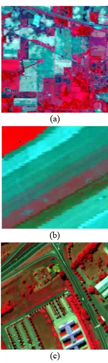
To assess the performance of the clustering algorithms three dataset are used in this study. The first hyperspectral image used in this study is acquired over Indiana’s Indian Pines region in 1992 by Airborne Visible/Infrared Imaging Spectrometer (AVIRIS). The image has dimension of 145×145 and consists of 220 bands, of which 20 bands falling in the water absorption region are removed. The ground reference image available with the image has 16 land cover classes. However in this study, ground reference image utilized by Paoli et al. (2009) and Li et al. (2013) is used. The modified ground reference image consists of five land cover classes, namely, wood, corn, grass, hay and soybean as shown in Figure 2 (a). The false color composite (FCC) of the Indian Pine image is shown in Figure 1 (a).
The second hyperspectral image used in this study is acquired over Valley of Salinas, Southern California in 1998 by AVIRIS. The image has dimension of 217×512 and consist of 220 bands, of which 20 bands falling in the water absorption region are removed. Spatial resolution of the image is 3.7 m. A subscene from the original image is also available for the analysis. Subscene named as Salinas-A has dimension of 83×86. The ground reference image for Salinas-A, available with the image, has six land cover classes. The ground reference image and land cover classes are shown in Figure 3 (a). The FCC of the Salinas-A image is shown in Figure 1 (b).
The third hyperspectral image used in this study is acquired over University of Pavia, northern Italy by ROSIS–03 optical sensor. The image has dimension of 610×340, consist of 103 bands and having spatial resolution of 1.3 m. A subscene of dimension 200×200 from the image is used in this study. According to the ground reference data available with the image, six out of the nine classes fall in 200×200 subscene. The ground reference image and land cover classes are shown in figure 4 (a). The FCC of the University of Pavia image is shown in Figure 1 (c).
4.1 Parameter Settings
ORCLUS requires two major parameters to be set by the users, which are, number of clusters (k ) and number of dimensions/bands (l). Also, algorithm requires value of k0 to
be set, which is nothing but the initial number of clusters seeds. It is very difficult to identify number of clusters without having any a priori knowledge about the dataset. In this study, the
value of k for both the dataset is decided by taking available ground reference image in to account. Hence, value of k for Indian Pines dataset is set to five and for Salinas-A and University of Pavia dataset it is set to six. Selecting optimum number of bands is a non trivial task. Generally, number of bands should be such that that the classes present in the image can be distinguished by the algorithm. Thus, if the image scene is complex and has large number of classes, then rationally more bands need to be selected (Du and Yang, 2008). Also, virtual dimensionality (Chang and Du, 2004) concept can be used to get some indication regarding number of bands to be selected. But in this study, value of l is empirically determined and for all the dataset l is set to 21. The value of k0 is set to
10k for all the datasets. For KM-SPCA algorithm number of clusters is similar to the value used by the ORCLUS k parameter.
(a)
(b)
(c)
Figure 1. FCC of (a) Indian Pines (R: 57, G: 27, B: 17), (b) Salinas-A (R: 57, G: 27, B: 17), and (c) University of Pavia (R: 102, G: 56, B: 31)
4.2 Results
The classified thematic maps and the ground reference image for Indian Pines dataset are shown in Figure 2 and the classification accuracies are reported in Table 1. It can be noted form Table 1 that out of the two algorithms, ORCLUS provides the best result. The main issue for both the algorithms is with identification of corn and soybean class. Many pixels of corn class are classified in soybean class and vice versa. Further, for KM-SPCA, hay class is problematic.
Wood Corn Grass
Hay Soybean
(a)
(b) (c) Figure 2. (a) Ground reference image of Indian Pines
dataset with color codes for different classes, and Classification maps obtained by (b) ORCLUS, (c) KM-SPCA.
Table 1. Various accuracy indicators obtained by the two clustering methods for Indian Pines dataset.
ORCLUS KM-SPCA
Wood UA 94.21 94.01
PA 66.54 75.84
Corn UA 38.02 41.16
PA 49.33 43.70
Grass UA 71.38 47.13
PA 89.95 92.24
Hay UA 77.54 0.00
PA 100 0.00
Soybean UA 71.63 71.05
PA 58.82 57.18
OA 65.83 55.66
Kappa 0.54 0.41
UA: User accuracy, PA: Producer accuracy, OA: Overall accuracy UA, PA & OA values are in percentage
The classified thematic maps and the ground reference image for Salinas-A dataset are shown in Figure 3 and the classification accuracies are reported in Table 2. It can be observed from Table 2 that both algorithms results in similar Kappa value. Careful observation of various class accuracies further reveals that, for all the classes, both the algorithms are behaving similarly. The similar behaviour can be attributed to the SPCA-image (dataset) interaction. Further investigations are required in this direction. Also from Table 2 it can be noted
that the main issue for both the algorithms is with the Corn_senesced_green_weeds class.
Brocoli_green_weeds_1
Corn_senesced_green_weeds
Lettuce_romaine_4wk
Lettuce_romaine_5wk
Lettuce_romaine_6wk
Lettuce_romaine_7wk
(a)
(b) (c) Figure 3. (a) Ground reference image of Salinas-A dataset
with color codes for different classes, and Classification maps obtained by (b) ORCLUS, (c) KM-SPCA.
Table 2. Various accuracy indicators obtained by the two clustering methods for Salinas-A dataset.
ORCLUS KM-SPCA
Brocoli_green_weeds_1 UA 100 100
PA 100 100
Corn_senesced_green_ weeds
UA 100 98.28
PA 26.13 25.68
Lettuce_romaine_4wk UA 51.41 51.59
PA 96.69 96.69
Lettuce_romaine_5wk UA 97.15 97.15
PA 100 100
Lettuce_romaine_6wk UA 83.12 80.38
PA 100 99.22
Lettuce_romaine_7wk UA 100 100
PA 98.53 96.32
OA 82.21 81.69
Kappa 0.78 0.78
UA: User accuracy, PA: Producer accuracy, OA: Overall accuracy UA, PA & OA values are in percentage
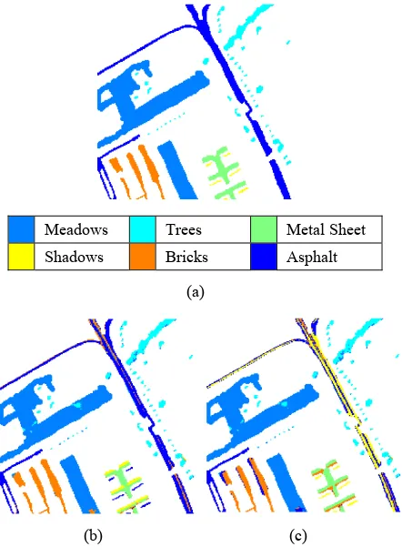
The classified thematic maps and the ground reference image for subscene of University of Pavia dataset are shown in Figure 4 and the classification accuracies are reported in Table 3. It can be observed form Table 3 that out of the two algorithms, ORCLUS provides the best result. The main issue for ORCLUS is with the identification of shadow class. ORCLUS is assigning all the pixels of shadow class to asphalt class. This behaviour can be explained as follows: due to small spatial presence of shadow class within the dataset, SPCA transformation is unable to preserve the sufficient information required to make the distinction between asphalt and shadow class, and thus to fill the vacant cluster, ORCLUS is dividing the class metal sheet into two classes. The class metal sheet is having a gabled roof structure and due to which side facing the sun and side not facing the sun are classified into two different clusters. For KM-SPCA major issue lies with the severe mixing of shadow and asphalt class.
Meadows Trees Metal Sheet
Shadows Bricks Asphalt
(a)
(b) (c)
Figure 4. (a) Ground reference image of University of Pavia dataset (200×200 subset) with color codes for different classes, and Classification maps obtained by (b) ORCLUS, (c) KM-SPCA.
5. CONCLUSION
In this study, unsupervised classification of hyperspectral imagery is carried out by using correlation clustering. As hyperspectral imagery is high dimensional data and suffers from “curse of dimensionality”, correlation clustering can be used to address these issues. The main advantage of correlation clustering algorithm lies in its ability to find subset of points (clusters) within a projected subspace and further, this projected subspace may differ for each cluster. For correlation clustering feature reduction method is tightly knitted with the clustering procedure. Instead of PCA, SPCA is interlaced with the
ORCLUS algorithm. Experiments are conducted on three real hyperspectral images. For all the dataset, performance of ORCLUS is acceptable. Major drawback lies in finding the appropriate values of the parameters. Although correlation clustering has appealing features for treatment of high dimensionality, but still more efforts and investigations are required to make it suitable for hyperspectral imagery.
Table 3. Various accuracy indicators obtained by the two clustering methods for subset of University of Pavia dataset.
ORCLUS KM-SPCA
Asphalt UA 89.78 81.82
PA 86.31 42.86
Meadows UA 97.17 97.06
PA 98.51 98.51
Trees UA 96.31 96.71
PA 89.70 88.41
Metal Sheet UA 100 99.03
PA 62.86 72.86
Shadows UA 0.00 16.26
PA 0.00 100
Bricks UA 74.14 70.33
PA 98.85 84.48
OA 90.17 82.78
Kappa 0.86 0.76
UA: User accuracy, PA: Producer accuracy, OA: Overall accuracy UA, PA & OA values are in percentage
ACKNOWLEDGEMENTS
The authors would like to thank Prof. David A. Landgrebe of Purdue University and Prof. Paolo Gamba of University of Pavia for making available the hyperspectral imagery used in this study. The first author [A.M.] thankfully acknowledges the financial support from the MHRD, India.
REFERENCES
Achtert, E., Kriegel, H-P. and Zimek, A., 2008. ELKI: a software system for evaluation of subspace clustering algorithms. In Proceedings of the 20th international conference on scientific and statistical database management (SSDBM), pp. 580-585.
Aggarwal, C.C., Wolf, J. L., Yu, P.S., Procopiuc, C. and Park, J. S., 1999. Fast algorithms for projected clustering. In Proceedings of the 1999 ACM SIGMOD international conference on Management of data, pp. 61-72.
Aggarwal, C.C. and Yu., P.S., 2000. Finding generalized projected clusters in high dimensional spaces. In Proceedings of the ACM SIGMOD international conference on management of data, pp. 70-81.
Beyer, K., Goldstein, J., Ramakrishnan, R. and Shaft, U., 1999. When is “nearest neighbor” meaningful? In Proceedings of the ISPRS Annals of the Photogrammetry, Remote Sensing and Spatial Information Sciences, Volume II-8, 2014
7th International Conference on Database Theory (ICDT), pp. 217-235.
Bilgin, G., Erturk, S. and Yildirim, T., 2011. Segmentation of hyperspectral images via subtractive clustering and cluster validation using one-class support vector machines. IEEE Transactions on Geoscience and Remote Sensing, 49(8), pp. 2936-2944.
Chang, C.-I. and Du, Q., 2004. Estimation of number of spectrally distinct signal sources in hyperspectral imagery. IEEE Transactions on Geoscience and Remote Sensing, 42(3), pp. 608-619.
Congalton R.G., 1991. A review of assessing the accuracy of classifications of remotely sensed data. Remote Sensing of Environment, 37(1), pp. 35-46.
Du, Q. and Yang, H., 2008. Similarity-Based Unsupervised Band Selection for Hyperspectral Image Analysis. IEEE Geoscience and Remote Sensing Letter, 5(4), pp. 564-568.
Jia, X. and Richards, J.A, 1999. Segmented principal components transformation for efficient hyperspectral remote-sensing image display and classification. IEEE Transactions on Geoscience and Remote Sensing, 37(1), pp. 538-542.
Kriegel, H-P., Kröger, P. and Zimek A., 2009. Clustering high-dimensional data: A survey on subspace clustering, pattern-based clustering, and correlation clustering. ACM Transactions on Knowledge Discovery from Data, 3(1), pp. 1-58.
Li, S., Zhang, B., Li, A., Jia, X., Gao, L. and Peng M., 2013. Hyperspectral Imagery Clustering With Neighborhood Constraints. IEEE Geoscience and Remote Sensing Letters, 10(3), pp. 588-592.
Mather P.M. and Koch M., 2011. Computer Processing of Remotely-Sensed Images: An Introduction, Fourth Edition, Wiley-Blackwell, Chichester, UK.
Niazmardi, S., Homayouni, S. and Safari, A., 2013. An Improved FCM Algorithm Based on the SVDD for Unsupervised Hyperspectral Data Classification. IEEE Journal of Selected Topics in Applied Earth Observations and Remote Sensing, 6(2), pp. 831-839.
Paoli, A, Melgani, F. and Pasolli, E., 2009. Clustering of Hyperspectral Images Based on Multiobjective Particle Swarm Optimization. IEEE Transactions on Geoscience and Remote Sensing, 47(12), pp. 4175-4188.
Richards, J. A., (2013). Remote Sensing Digital Image Analysis, Springer, Berlin Heidelberg.
Sim, K., Gopalkrishnan, V., Zimek, A. and Cong, G., 2013. A survey on enhanced subspace clustering. Data Mining and Knowledge Discovery, 26(2), pp. 332-397.
Villa, A., Chanussot, J., Benediktsson, J.A., Jutten, C. and Dambreville, R., 2013. Unsupervised methods for the classification of hyperspectral images with low spatial resolution. Pattern Recognition, 46(6), pp. 1556-1568.