PLEASE SCROLL DOWN FOR ARTICLE
On: 8 December 2008Access details: Access Details: [subscription number 778576936] Publisher Routledge
Informa Ltd Registered in England and Wales Registered Number: 1072954 Registered office: Mortimer House, 37-41 Mortimer Street, London W1T 3JH, UK
Journal of the Asia Pacific Economy
Publication details, including instructions for authors and subscription information: http://www.informaworld.com/smpp/title~content=t713703356
FDI and environmental regulations in China
Jing Zhang a; Xiaolan Fu ba Department of Economics, University of Birmingham, UK b Department of International Development, University of Oxford, UK
Online Publication Date: 01 August 2008
To cite this Article Zhang, Jing and Fu, Xiaolan(2008)'FDI and environmental regulations in China',Journal of the Asia Pacific Economy,13:3,332 — 353
To link to this Article: DOI: 10.1080/13547860802131326 URL: http://dx.doi.org/10.1080/13547860802131326
Full terms and conditions of use: http://www.informaworld.com/terms-and-conditions-of-access.pdf This article may be used for research, teaching and private study purposes. Any substantial or systematic reproduction, re-distribution, re-selling, loan or sub-licensing, systematic supply or distribution in any form to anyone is expressly forbidden.
Vol. 13, No. 3, August 2008, 332–353
FDI and environmental regulations in China
Jing Zhanga,∗and Xiaolan Fub
aDepartment of Economics, University of Birmingham, UK;bDepartment of International Development, University of Oxford, UK
This paper uses provincial socioeconomic and environmental data and investi-gates whether there exists an intra-county pollution haven effect for China. We examine whether differences in the stringency of environmental regulations affect the choice of location for FDI in China. We use a five-year panel dataset for 30 provinces in China that includes three measures of environmental reg-ulations, which vary across time and province, and a significant number of control variables including measures of agglomeration and factor abundance. We control for unobserved heterogeneity by using a feasible generalised least square estimator. Our results suggest that environmental stringency has a significant and negative effect on FDI, leading us to conclude that, ceteris paribus, FDI prefers to locate into regions with relatively weak environmental regulations. This provides some support for the existence of a pollution haven within China.
Keywords:FDI; environmental regulations; pollution haven hypothesis
JEL Classifications:F21, O13, Q58
Introduction
Traditional international trade theory tells us that trade is governed by comparative advantage, which postulates that the efficient exchange of goods leads to optimal outcomes. Multinational firms, as agents of free trade, seek cost reductions and respond to market imperfections. Higher domestic costs therefore provide the motivation for multinational corporations to expand their geographical range into other areas. Such a strategy could trigger competition for lax environmental poli-cies in order to gain competitive advantage in ‘dirty’ goods production. A corollary is that developing countries may join a ‘race to the bottom’ by undervaluing envi-ronmental damage in order to attract more FDI. Either way, the result is excessive levels of pollution and environmental degradation (Deanet al.2005). This is the so-called pollution haven hypothesis.
To date, one of the most contentious debates in the FDI and the environ-ment literature focuses on whether inter-country differences in environenviron-mental
∗Corresponding author. Email: jxz305@bham.ac.uk ISSN: 1354-7860 print / 1469-9648 online
C
2008 Taylor & Francis DOI: 10.1080/13547860802131326 http://www.tandf.co.uk/journals
regulations are turning poor countries into ‘pollution havens’. This argument centres on the cost effectiveness of environmental regulations and presumes that there are environmental-regulation induced production cost differentials that encourage a firm to relocate its production facility. Theoretical mod-els of pollution havens, including Pearson (1987) and Baumol and Oates (1988), illustrate that developed countries control pollution emissions whilst developing countries do not, and hence become pollution havens. However, the empirical evidence from testing the pollution haven hypothesis (PHH) is mixed.
Deanet al.(2005) and Javorcik and Wei (2005) divide the existing PHH lit-erature into three strands: (1) intra-country, inter-region plant location choice; (2) inter-industry FDI flows within a country and; (3) inter-country FDI loca-tion choice. Using the first approach, Levinson (1996) employs a condiloca-tional logit model and finds little evidence that inter-state differences in environ-mental regulations affect the US plant location choice. A similar approach is adopted by List and Co (2000) who estimate the effect of state environmen-tal regulations on foreign multinational corporations’ new plant location deci-sions from 1986 to 1993, and find that environmental stringency and attrac-tiveness of a location are inversely related. Keller and Levinson (2002) test whether FDI to US states has responded significantly to relative changes in state’s environmental compliance costs. They robustly document moderate ef-fects of pollution abatement costs on capital and employees at foreign-owned manufacturing affiliates, particularly in pollution-intensive industries, and on the number of planned new foreign-owned manufacturing facilities. Similarly, Fredriksson et al. (2003) use US state-level panel data from four industrial sectors over the period 1977–1987, and find that environmental policy plays a significant role in determining the spatial allocation of inbound US FDI and such an effect depends critically on the exogeneity assumption of environmental policy.
A recent study that provides empirical evidence for intra-country pollution havens in China is Deanet al.(2005). They estimate whether weak environmental regulations attract foreign investment in China. They construct a location choice model containing firm’s production and abatement decisions, agglomeration and factor abundance, and estimate a conditional logit model. Their results show that FDI flows to provinces with high concentrations of foreign investment, relative abundance of skilled labour, concentration of potential local suppliers, special tax incentives, and less state ownership. Environmental stringency only affects certain types of projects in highly polluting industries, with investment originating from Hong Kong, Macau and Taiwan seemingly being attracted to provinces with relatively weak environmental controls. This finding is consistent with the pollution haven hypothesis but contradicts the notion that pollution havens are generated by industrial country investors. This is opposite to the pollution haven hypothesis. In sum, the results suggest little evidence for the pollution haven hypothesis.
There is a scarcity of research that assesses the relationship between the distribution of foreign investment and pollution intensity. One exception is the recent work by Eskeland and Harrison (2003) who adopt the inter-industry analysis approach to examine the pattern of FDI across industries in Mexico, Venezuela, Morocco and Cˆote d’Ivoire. Their results suggest that it is difficult to find a robust relationship between pollution abatement and the volume of US outbound investment. They find a positive relationship between FDI share and air pollution-intensity of an industry but negative relationship between FDI share and both water pollution and toxic release-intensity. It is suggested that these results are because pollution abatement costs are only a small fraction of overall costs.
A paper employing the inter-country analysis approach is Xing and Kolstad (2002) which presents a statistical test on how US FDI is influenced by the environmental regulations of foreign host countries. The results show that the laxity of environmental regulations in a host country is a significant determinant of FDI from the US for heavily polluting industries and is an insignificant determinant of FDI from the US for less polluting industries. Their findings provide indirect support to the pollution haven hypothesis. However, the small size of the data and imperfect coverage of sulphur emissions data mean that care must be taken with the reliability of their results. A more recent paper by Javorcik and Wei (2005) examines the relationship between cross-country FDI flows and environmental stringency for 143 multinational firms in 25 countries in Eastern Europe and the former Soviet Union. They find some evidence for the PHH in regressions employing treaties as a proxy for environmental standards in a host country, but the overall evidence is relatively weak and does not survive numerous robustness checks using other proxies of pollution intensity or regulatory stringency.
On balance, the previous empirical studies find little evidence to support the pollution haven hypothesis and the general lack of such results can be summarised as follows. First, as Pearson (1987, p. 124) pointed out, ‘environmental control costs are a small fraction of production costs in virtually every industry, and the effect on trade will be correspondingly small’. Second, FDI may be combined with new techniques, including the latest pollution abatement technologies, rendering the relative stringency of the host country’s environmental regulations unimportant. If firms are producing for export, then they may have to meet the environmental product standards of developed countries to be able to gain the access to these markets. And finally, firms may predict that there will be future increases in environmental regulations, and hence choose a production process today that will meet the higher standards of the future (Deanet al. 2002).
There are also a number of issues arising with regards to the econometric estimation of models for the PHH. First, in some studies, the absence of some im-portant variables, such as relative factor abundance and agglomeration, will lead to omitted variable bias. Markusen and Zhang (1999), Head and Ries (1996), Cheng and Kwan (2000) have demonstrated the importance of these variables in explain-ing FDI incidence (Deanet al. 2005). Second, it is difficult to quantify international differences in environmental regulations (Keller and Levinson 2002; Javorcik and
Wei 2005). Third, Keller and Levinson (2002) and Levinson and Taylor (2008) both demonstrate that cross-section analyses cannot control for unobserved hetero-geneity among countries. The unobserved characteristics, such as unobserved re-sources and unobserved protection of polluting industries, may be correlated with both regulatory compliance costs and investment. Therefore, use of a continuous, time-varying (panel) dataset becomes important. Finally, most literature uses cost-based measures of environmental standard stringency. Copeland and Taylor (2003) develop a model linking the firm’s production and abatement cost. The model sug-gests a particular specification for testing the firm’s responsiveness to changes in environmental regulations, which raises the possibility of specification error.
China has, in recent years, become one of the largest recipients of worldwide foreign direct investment (FDI) with inflows of $72 billion in 2005. However, there remains a significant disparity in the geographical distribution of FDI in-flows into China. In the mean time, environmental deterioration has become a serious problem associated with rapid economic growth in China, and industrial pollutant emissions are a major cause of the environmental problem. Pollution emissions vary across the Chinese regions, and the strength of the enforcement of the environmental regulations varies across regions. There have been considerable studies investigating the determinants of FDI location choice in China. Labour costs, potential market size, market access, supplier access, infrastructure, pro-ductivity, education levels, preferential policies, and spatial dependence are found to have affected the regional distribution of FDI in China (e.g. Coughlin and Segev 2000; Cheng and Kwan 2000; and Amiti and Javorcik, 2008). However, these stud-ies all omitted certain structural determinants of FDI, for example, environmental regulation stringency.
In this paper, we address a number of those limitations and investigate whether there exists an intra-county pollution haven effect for China. We adopt a five year-panel dataset for 30 provinces in China that includes three measures of envi-ronmental regulations that vary across time and province, and a significant number of control variables including measures of agglomeration and factor abundance. We control for unobserved heterogeneity by using feasible generalised least square estimator. Our results suggest that environmental stringency has a significant neg-ative effect on FDI, leading us to conclude that, ceteris paribus, FDI prefers to locate into regions with relatively weak environmental regulations and provides some support for the existence of a pollution haven within China.
The paper is organised as follows. The next section describes FDI inflows into China and China’s environment problems and environmental regulation system. The section after presents our methodology and data, and the fourth section reports and discusses the empirical results. The final section concludes.
FDI, the environment and environmental regulations in China
Since it launched economic reforms in 1978, China has received enormous FDI flows. General trends and the characteristics of FDI in China have been reviewed
by many studies, for example Wu (1999), OECD (2000). At the beginning of China’s economic reforms, FDI inflows were not significant. FDI increased in the mid-1980s and reached a peak level in the early 1990s. From 1994, the growth rate of FDI slowed down and became negative in 1999. From 2000 onwards, inflows of FDI into China recovered quickly. In 2003, it overtook the US as the biggest recipient of FDI in the world with an actually used value of $53.51 billion.
Although the total amount of FDI inflows into China are extremely high, there are significant imbalances in FDI stocks across China in terms of their source, form, geographical and sectoral distribution. According to the report from China’s Ministry of Commerce, Asian countries contributed most of the FDI inflows into China, constituting more than 70% of total actually used FDI in China between 1979 and 2003. They are followed by North America and the EU, with 9.57% and 7.55% respectively. With regards to the forms of investment, the establishment of new enterprises like joint ventures and foreign-invested companies seem to be the main forms of FDI into China at the current time. Thirdly, the geographical distribution of FDI in China is very imbalanced. Eastern regions have received most of the FDI inflows. 86.27% of cumulative FDI was located in the eastern region, 8.93% in the central region and only 4.80% in the western region between the years 1979 and 2003. And finally, the majority of FDI has flowed into the secondary industry.1 Among secondary industries, manufacturing attracted 63.66% of the total cumulative contracted FDI by 2003.
China is a large polluting country with rapidly increasing industrial production, domestic and foreign trade and investment. Manufacturing is the primary source of the environmental problems. The State Environmental Protection Administration (SEPA) reported that, in 2004, industrial air pollution accounted for over 80% of the national total. Although industrial water pollution has decreased year by year, it still accounts for about 45.8% of national total.
Faced with such serious environmental problems, China’s central and local governments, as well as some enterprises, have invested a great amount of money for environmental pollution treatment every year. Figure 1 shows the rising trend of investments in industrial pollution treatment from 1987 to 2004. Figure 2 shows that the provincial share of pollution treatment investment relative to GDP varies across province, an imbalance that is not consistent with GDP levels.
Environmental protection in China became the responsibility of the country in 1978, based on the Constitution of the People’s Republic of China. China estab-lished the Environment Protection Law (EPL) in 1979 (provisional), and officially enacted it in September 1989. The EPL provides the basic principles governing the prevention of pollution and environmental pollution and imposes criminal re-sponsibility for serious environmental pollution. The effort of the government on environmental protection is ongoing. In 2006, Chinese Premier Wen Jiabao pointed out the importance of green development in his government work report (Reuters, 16/08/2006). Generally, there are no separate environmental standards for foreign investment, but foreign investors’ environmental behaviour must abide by Chinese environmental laws and regulations and meet the environmental standards.
0.00 5.00 10.00 15.00 20.00 25.00 30.00 19 87 19 88 19 89 19 90 19 91 19 92 19 93 19 94 19 95 19 96 19 97 19 98 19 99 20 00 20 01 20 02 20 03 In v e st m e n t Year
Investment in Industrial Pollution Treatment
Investment in Industrial Pollution Treatment (billion RMB)
Figure 1. Investment in industrial pollution treatment 1987–2004. Source: China Statistical Yearbook, various years.
Although the regulatory framework seems comprehensive, the enforcement is weak. Ma (2007) points out that the limited power of environmental authorities is one reason for the failure to implement environmental law. Environmental policy is set by the government, overseen by the environmental authorities and imple-mented by various government departments. The coordination between the envi-ronmental authorities and other departments is poor. Excessive pollution happens in some regions due to the failure of local government. As a result, regulatory strength varies significantly across regions. The weak environmental regulatory stringency in China provides an opportunity for some multinational firms to take advantage of weak environmental standards to transfer their out-of-date technolo-gies and pollution-intensive production to China.
Methodology
We follow the methodology of previous studies on intra-country, inter-region FDI location choice and investigate the interaction between FDI flows and environ-mental regulations in China.
Estimating model and data
Multinational corporations (MNCs) are assumed to seek to maximise profit, i.e. to minimise costs. A MNC will view and compare different locations to assess dif-ferences in, for example, production costs, government regulations, infrastructure,
338 J. Zhang and X. Fu Beijing Tianjin Hebei Shanxi Inner Mongolia Liaoning Jilin Heilongjiang Shanghai Jiangsu Zhejiang Anhui Fujian Jiangxi Shandong Henan Hubei Hunan Guangdong Guangxi Hainan Chongqing Sichuan Guizhou Yunnan Tibet Shaanxi Gansu Qinghai Ningxia Xinjiang 0.0 0.1 0.2 0.3 0.4 0.5 0.6 0.7 0.8 0.9 1.0 1.1 1.2
0 200 400 600 800 1000 1200 1400 1600 1800
Po ll u tio n Tre a tm en t I n v e st m en t / G D P (% )
Provincial GDP (billion yuan)
Pollution Treatment Investment/GDP and Provincial GDP
agglomeration effects and so on. When considering the impact of environmental regulations on foreign plant location choice, the empirical model that is adopted in this paper is given by
F DIit =α+β1ERit+β2Xit+ηi+γt+εit (1)
where,
FDIis the amount of FDI inflow into regioniin time periodt; ERis the vector of measures to capture environmental stringency; Xis the set of other regional characteristics that may affect FDI; ηis time-invariant regional effects;
γis location-invariant time effects; and εis the idiosyncratic error term.
We employ two variables to capture FDI inflows, one of which is the value of FDI divided by regional GDP (FDI/GDP) and the other is FDI divided by regional population (FDI/POP). Scaling FDI by GDP or population allows FDI to be comparable across regions and time (see Appendix 1 for variable definitions and sources).
Factors that may influence provincial level FDI include environmental strin-gency, factor prices, infrastructure, and agglomeration effects. The level of envi-ronmental stringency in different provinces is proxied by three variables:
r
EI1– the share of investment in industrial pollution treatment projects in total innovation investment. Industrial pollution treatment investment is the total investment of enterprises in construction and installation projects, and purchase of equipment and instruments required in the pollution harnessing projects for the treatments of wastewater, waste gas, solid wastes, noise pollution and other pollution.We use the share of industrial pollution treatment investment in innovation investment to reflect the local government effort in environmental protection. We also normalise the industrial pollution treatment investment using two other methods (see details in Appendix 2).
r
Punish – the total number of administrative punishment cases filed by the envi-ronmental authorities in each region normalised by the number of enterprises in each region.2Administrative punishment cases are those cases that breach environmental protection laws and regulations. Punish proxies the strength of enforcement of regional environmental legislation.r
Charge – a pollution emission charge normalised by the number of organisa-tions that paid this charge. The pollution emission charge refers to the total amount of (1) pollutant emission charge exceeding the discharge standards; (2) sewage discharge levy; and (3) four other kinds of charges, i.e. increasing levy standards, double charges, overdue charges and compensation fines. Thepollution charge is implemented by regional governments and reflects the provincial differences in implementation of the pollution levy system.
These three measures are time varying, which improves upon the 0–3 type of measure of environmental stringency used in Javorcik and Wei (2005). Since more stringent environmental regulations will generate higher pollution taxes or higher pollution abatement costs for the firm, the environmental regulation stringency variables should have a similar impact to factor prices on foreign investment location choice. It is expected that FDI is attracted to provinces with weaker regulations, i.e. with a lower share of investment in industrial pollution treatment investment, with a lower number of normalised administrative punishment cases related to environmental issues, and/or with a lower normalised pollution emission charge. Since the pollution emission charge is more visible to enterprises than administrative punishment cases and environmental investment, we expect Charge has the strongest impact on FDI location choice, followed by Punish and EI1, respectively.
Our control variables are as follows.
Manufacturing wage is included as a proxy for factor price differences across each region. The quality of labour force in a region is captured by two measures, labour productivity and the illiteracy rate. Population density is employed as a proxy for land prices and potential market size (assuming that labour mobility between provinces is low). The availability and quality of infrastructure also impacts the overall cost of doing business and hence is an attractive factor to FDI location. We include both railway density and road density to measure the quality of the regional transportation network and thus to proxy the cost and availability of material inputs. Gross regional product (GRP) per capita is included to capture the average quality of the government, general infrastructure and the effect of market size differences across regions. The regional gross industrial product value (GIP) attempts to capture an agglomeration effect whereby firms locate where hubs of economic activity already exist (Bartik 1988). GIP may also be an indicator of availability of intermediate inputs.
Following the literature, foreign investors are seeking a location with compar-ative advantages such as cheaper factors that they use in higher proportions. Since unskilled labour is associated with lower labour costs, FDI is also expected to be attracted to provinces with relatively lower manufacturing wages. Some recent empirical studies on intra-country FDI flows find significant negative effects of wage on aggregate FDI flows in China (e.g. Coughlin and Segev 2000; and Cheng and Kwan 2000). Conversely, wage is also found to be positively related with FDI flows (Gao 2002). To specify the real impact of wage on FDI inflows, we add wage squared in our estimations and expect an inverted-U relationship be-tween FDI and wage. When wage is below some benchmark, foreign investments are attracted to provinces with high wage level because labour cost is not the most important determinant compared with other factors, such as high regional income and good infrastructure. But when wage is higher than the benchmark,
FDI is deterred because wage becomes more important in the standard profit function.
According to the previous work of Head and Ries (1996) and Dean et al. (2005), it expected that FDI would like to flow into provinces with better industrial agglomeration and infrastructure. In addition, for foreign investors seeking a large local market they may be expected to invest in areas that have a large consumption capability and potential, which can be proxied by population density and per capita income. However, population density also proxies land price. In more densely populated areas, land price is usually higher than that in less densely populated areas. The sign of population density is expected to be ambiguous.
Our five-year time period panel data help to control for unobserved hetero-geneity. Since the independent variables do not have an immediate influence on the investment location choice, we employ a one-year lag for all independent variables. The lagged independent variables also help to control for the possible endogeneity of these variables. Therefore, the estimating equation is:
ln (F DIit)=α+β1ln (ERit−1)+β2ln (GRP per Capit ait−1)
+β3ln (W ageit−1)+β4(ln (W ageit−1))2+β5ln (GI Pit+1) +β6ln (P op. Densityit−1)+β7ln (Rail Densityit−1) +β8ln (Road Densityit−1)+β9ln (I llit erat e Rat eit−1) +β10ln (P roduct ivityit−1)+ηi+γt+εit (2)
wherei refers to province, and t refers to year. We use the log transformation models, which could help to correct the positive skewness of variables and make the error term close to homoskedestic.3
If there is no effect of the stringency of environmental regulations on FDI across regions, we would expectβ1=0. Ifβ1<0, we cannot reject the hypothesis that FDI is attracted to provinces with lower regulatory stringency. The expected signs of the coefficients are as follows:
Coefficients β1 β2 β3 β4 β5 β6 β7 β8 β9 B10
Expected Signs − + + − + −/+ + + + −
Data used for this study are collected from the China Statistical Yearbook, China Industrial Economy Statistical Yearbooks and China Environment Yearbook. The values of all the data are deflated by the GDP deflator, which is set to 100 for year 1990. All the FDI data, which are measured by US dollars, are transferred to RBM yuan at the middle exchange rate of the year. A complete description of definitions of all variables and sources is provided in Appendix 1. Because one year lags are used for all independent variables in the estimation, all the socioeconomic
independent variables of 30 regions are from 1998 to 2002. FDI data used for estimations are therefore from 1999 to 2003.4
To gauge the consistency of the sample with what is known about the provin-cial distribution of foreign investment, we compare the provinprovin-cial shares of total actually used FDI value in the sample. It is seen that the largest FDI inflows went to eastern regions/provinces. The values of our three environmental stringency variables vary widely across provinces, and a province could appear to be strin-gent using one measure of environmental regulations but not using the others. The correlation matrix (see Table 1) shows that these three environmental stringency variables do not have a strong correlation. The correlation matrix also shows that our FDI variables seem to have a negative correlation with EI1and Punish, but a positive correlation with Charge. The correlations between the two FDI variables and other independent variables implies that FDI prefers to flow into provinces with better infrastructure, higher population density, higher income level, better agglomeration, higher quality of labour and higher labour costs.
Selection of estimators
A problem faced when estimating the model is whether the unobserved individual-specific effects and time effects (ηiandγt) should be treated as random variables or as parameters to be estimated for each cross-region observationiand timet. In this paper, we estimate both two-way fixed effects and random effects error com-ponent models. For our fixed effects models we initially use the within regression estimator which is a pooled OLS estimator based on time-demeaned variables, or use the time variation in both dependent and independent variables within each cross-sectional observation (Wooldridge 2000). For our random effects models we choose the generalised least square (GLS) estimator, which produces a matrix-weighted average of the between and within estimator results.5
Few assumptions are required to justify the fixed effects estimator. In the estimation, however,ηi andγt are not assumed to have a distribution, but are treated as fixed and estimatable. The random effects estimator requires no corre-lation assumptions, that isηi ∼IID (0,ση2),γt ∼IID (0,σγ2), andεit ∼IID (0, στ2) are independent of each other. In addition, all the independent variables are independent ofηi,γt, andεitfor alliandt.
In order to calculate whetherεit are uncorrelated with the independent vari-ables, we use the Hausman specification test under the null hypothesis H0: E(εit|Xit)=0. The results of Hausman specification tests suggest that, in most cases, the individual-level effects could be adequately modelled by random effects models.6
We presume that all the one-year lagged control variables are exogenous. However, environmental regulation stringency may be endogenous partly because the regions with relatively low FDI inflows may lower their environmental reg-ulation standards in order to attract more FDI, and partly because FDI is an important engine of growth and hence helps to improve regional environment and
Journal
of
the
A
sia
P
acific
Econom
y
343
Table 1. Correlations of the variables.
FDI/ GDP
FDI/ POP EI1 1
Punish 1
Charge 1
GRP per capita
1 Wage 1 (Wage
1)2 GIP 1 Pop. Density
1
Rail Density
1
Road Density
1
Illiterate
Rate 1 Productivity 1
FDI/GDP 1.000 FDI/POP 0.859 1.000 EI1 1 −0.095 −0.120 1.000 Punish 1 −0.108 −0.113 0.154 1.000 Charge 1 0.294 0.601 0.060 −0.014 1.000 GRP per capita 1 0.617 0.904 −0.084 −0.029 0.700 1.000 Wage 1 0.511 0.781 −0.108 −0.062 0.568 0.862 1.000 (Wage 1)2 0.475 0.791 −0.134 −0.108 −0.162 −0.083 0.654 1.000 GIP 1 0.544 0.553 0.019 −0.027 0.409 0.488 0.433 0.409 1.000 Pop. Density 1 0.502 0.807 −0.143 −0.157 0.801 0.865 0.674 0.742 0.429 1.000 Rail Density 1 0.393 0.616 −0.010 0.007 0.465 0.723 0.555 0.571 0.120 0.606 1.000 Road Density 1 0.697 0.798 −0.098 −0.173 0.538 0.771 0.695 0.701 0.456 0.729 0.723 1.000
Illiterate Rate 1 −0.321 −0.353 0.004 −0.229 −0.150 −0.421 −0.345 −0.322 −0.266 −0.279 −0.451 −0.430 1.000
environmental standards. We employ a Davidson–MacKinnon test of the exogene-ity using two-year lagged environmental regulation variables as the instrumental variable. The results suggest that simultaneity bias is not present in our model for all three environmental regulation variables.
When using data on different provinces that have a variation of scale, the variance for each of the panels will differ. Both the fixed effects and random effects estimators can solve the problem of heteroscedasticity across panels. However, neither controls for possible autocorrelation within the panels. In order to test whether the errors suffer from autocorrelation or not, we apply the following dynamic regression model:
εit =ρεit−1+νit, t=2, . . . , T (3)
where|ρ|<1 andνit ∼IID(0,σν2).
The null hypothesis is H0: ρ = 0. Thus, ρ should be estimated from the regression ofεit onεit−1, for allt =2,. . .,T. Thet statistics for ˆρ show that we can reject the null hypothesis for all log models. That is, there is AR (1) autocorrelation within panels in our log specifications.
One solution is to use the feasible generalised least square (FGLS) estima-tor. FGLS models allow cross-sectional correlation and heteroscedasticity. It also allows models with heteroscedasticity and no cross-sectional correlation. In addi-tion, it is possible to relax the assumption of non-autocorrelation within panels. FGLS is therefore more efficient than the other two estimators mentioned above.7 Since the GLS estimator is less efficient than the FGLS estimator, the random effects results are relatively weak even though the GLS estimator is not rejected in most specifications by Hausman specification tests.8We therefore concentrate on the FGLS estimation results in the main text. Estimations are run using STATA 9.9
Empirical results
In this section we only report the FGLS log results because of its advantages mentioned above. We also include a series of sensitivity checks.10
Tables 2–4 respectively present the FGLS regression results for the impact of different levels of environmental stringency on two measures of provincial level FDI inflows using data in logs for 30 provinces in China. Table 2 presents the results for EI1, Table 3 for Punish and Table 4 for Charge. Each table includes two parts, depending on the two measures of FDI inflows, FDI/GDP for columns 1–4 and FDI/POP for columns 5–8.
The results in Table 2 show that the share of industrial pollution treatment in-vestment has a negative and significant effect on FDI inflows into a province. The coefficients are relatively stable across regressions. The coefficients in columns (4) and (8) indicate that for both measures of FDI, a 10% increase in the share of environmental investment of a province would lead to a 0.62% decrease in the amount of FDI inflows into the province. Thus, the more stringent are the
Journal
of
the
A
sia
P
acific
Econom
y
345
Table 2. FGLS regression results for log data with EI1.
FDI/GDP FDI/POP
(1) (2) (3) (4) (5) (6) (7) (8)
EI1 1 −0.087 −0.11 −0.063 −0.062 −0.094 −0.10 −0.062 −0.062
(−2.69)∗∗∗ (−3.16)∗∗∗ (−2.00)∗∗ (−2.03)∗∗ (−2.75)∗∗∗ (−2.93)∗∗∗ (−1.93)∗ (−1.96)∗∗
GRP per capita 1 2.82 3.48 3.41 3.44 3.43 3.99 4.04 3.98
(4.03)∗∗∗ (4.66)∗∗∗ (4.98)∗∗∗ (4.86)∗∗∗ (4.93)∗∗∗ (5.42)∗∗∗ (6.04)∗∗∗ (5.74)∗∗∗
Wage 1 5.76 3.22 5.34 6.49 7.95 5.53 7.48 8.54
(1.56) (0.81) (1.45) (1.68)∗ (2.24)∗∗ (1.41) (2.03)∗∗ (2.22)∗∗
Wage 12 −0.33 −0.19 −0.32 −0.40 −0.46 −0.32 −0.45 −0.52
(−1.48) (−0.78) (−1.44) (−1.71)∗ (−2.11)∗∗ (−1.36) (−2.01)∗∗ (−2.24)∗∗
GIP 1 −0.60 −0.25 −0.16 −0.42 −0.057 0.045
(−2.00)∗∗ (−0.80) (−0.50) (−1.31) (−0.18) (0.13)
Pop. Density 1 −1.14 −1.01 −1.13 −0.96 −0.88 −0.92
(−1.50) (−1.49) (−1.68)∗ (−1.25) (−1.21) (−1.28)
Rail Density 1 −0.21 −0.25 −0.16 −0.20
(−1.98)∗∗ (−2.32)∗∗ (−1.43) (−1.78)∗
Road Density 1 0.42 0.45 0.45 0.47
(4.14)∗∗∗ (5.30)∗∗∗ (4.47)∗∗∗ (5.47)∗∗∗
Illiterate Rate 1 0.27 0.27
(2.34)∗∗ (2.23)∗∗
Productivity 1 −0.18 −0.17
(−1.47) (−1.34)
Constant −44.122 −27.27 −40.74 −43.51 −59.51 −44.54 −58.28 −60.91
(−2.45)∗∗ (−1.28) (−2.11)∗∗ (−2.20)∗∗ (−3.43)∗∗∗ (−2.10)∗∗ (−2.96)∗∗∗ (−3.05)∗∗∗
Waldχ2 5384.91 5717.34 7051.28 7071.95 8913.67 9316.90 12471.36 13239.35
Observations 149 149 149 149 149 149 149 149
346
J.
Zhang
and
X.
Fu
Table 3. FGLS regression results for log data with Punish.
FDI/GDP FDI/POP
(1) (2) (3) (4) (5) (6) (7) (8)
Punish 1 −0.051 −0.078 −0.082 −0.076 −0.054 −0.074 −0.078 −0.070
(−2.13)∗∗ (−3.01)∗∗∗ (−3.16)∗∗∗ (−2.85)∗∗∗ (−2.26)∗∗ (−2.57)∗∗ (−2.62)∗∗∗ (−2.38)∗∗
GRP per capita 1 3.13 3.79 3.84 3.85 3.63 4.28 4.46 4.36
(4.51)∗∗∗ (5.13)∗∗∗ (5.94)∗∗∗ (5.75)∗∗∗ (5.34)∗∗∗ (5.79)∗∗∗ (6.99)∗∗∗ (6.58)∗∗∗
Wage 1 5.42 3.41 4.78 5.73 7.63 5.54 6.64 7.67
(1.35) (−0.81) (−1.24) (−1.42) (1.98)∗∗ (1.33) (1.72)∗ (1.91)∗
Wage 12 −0.33 −0.21 −0.30 −0.36 −0.45 −0.34 −0.41 −0.47
(−1.36) (−0.84) (−1.28) (−1.48) (−1.92)∗ (−1.33) (−1.73)∗ (−1.94)∗
GIP 1 −0.62 −0.41 −0.36 −0.48 −0.20 −0.13
(−1.98)∗∗ (−1.36) (−1.17) (−1.40) (−0.63) (−0.39)
Pop. Density 1 −0.94 −0.98 −1.02 −0.69 −0.82 −0.77
(−1.26) (−1.57) (−1.63) (−0.90) (−1.18) (−1.13)
Rail Density 1 −0.30 −0.31 −0.26 −0.26
(−2.87)∗∗∗ (−2.90)∗∗∗ (−2.25)∗∗ (−2.28)∗∗
Road Density 1 0.44 0.46 0.46 0.48
(4.44)∗∗∗ (5.28)∗∗∗ (4.72)∗∗∗ (5.43)∗∗∗
Illiterate Rate 1 0.21 0.20
(1.83)∗ (1.68)∗
Productivity 1 −0.16 −0.14
(−1.32) (−1.14)
Constant −44.12 −31.19 −39.87 −42.58 −58.88 −47.77 −56.75 −59.97
(−2.30)∗∗ (−1.40) (−2.00)∗∗ (−2.10)∗∗ (−3.19)∗∗∗ (−2.16)∗∗ (−2.80)∗∗∗ (−2.92)∗∗∗
Waldχ2 4945.25 6263.02 8235.71 8466.13 8280.40 8852.64 13005.62 13589.33
Observations 147 147 147 147 147 147 147 147
Journal
of
the
A
sia
P
acific
Econom
y
347
Table 4. FGLS regression results for log data with Charge.
FDI/GDP FDI/POP
(1) (2) (3) (4) (5) (6) (7) (8)
Charge 1 −0.12 −0.14 −0.22 −0.18 −0.098 −0.13 −0.21 −0.17
(−1.01) (−1.16) (−2.00)∗∗ (−1.54) (−0.84) (−1.10) (−1.92)∗ (−1.50)
GRP per capita 1 2.89 3.47 3.50 3.47 3.57 3.99 4.15 4.02
(3.95)∗∗∗ (4.42)∗∗∗ (5.02)∗∗∗ (4.80)∗∗∗ (4.95)∗∗∗ (5.25)∗∗∗ (6.27)∗∗∗ (5.77)∗∗∗
Wage 1 3.87 0.49 1.99 3.26 6.69 3.02 4.18 5.47
(0.94) (0.11) (0.49) (0.77) (1.67)∗ (0.67) (1.02) (1.29)
Wage 12 −0.23 −0.039 −0.12 −0.20 −0.39 −0.19 −0.25 −0.33
(−0.90) (−0.14) (−0.48) (−0.78) (−1.59) (−0.68) (−0.99) (−1.28)
GIP 1 −0.31 0.13 0.14 −0.15 0.30 0.34
(−0.94) (0.39) (0.42) (−0.45) (0.89) (0.97)
Pop. Density 1 −1.39 −1.54 −1.61 −1.22 −1.42 −1.41
(−1.67)∗ (−2.27)∗∗ (−2.34)∗∗ (−1.45) (−1.92)∗ (−1.92)∗
Rail Density 1 −0.37 −0.37 −0.31 −0.31
(−3.45)∗∗∗ (−3.34)∗∗∗ (−2.69)∗∗∗ (−2.68)∗∗∗
Road Density 1 0.42 0.44 0.45 0.46
(3.92)∗∗∗ (4.46)∗∗∗ (4.20)∗∗∗ (4.57)∗∗∗
Illiterate Rate 1 0.22 0.21
(1.68)∗ (1.58)
Productivity 1 −0.16 −0.16
(−1.32) (−1.25)
Constant −35.64 −14.44 −24.28 −27.59 −54.22 −32.42 −42.16 −45.52
(−1.81)∗ (−0.60) (−1.15) (−1.29) (−2.81)∗∗∗ (−1.36) (−1.96)∗∗ (−2.09)∗∗
Waldχ2 4558.54 4891.34 7336.94 6817.20 7749.89 8301.63 12585.14 12082.78
Observations 149 149 149 149 149 149 149 149
environmental regulations the lower is the amount of FDI. Per capita income gen-erally has a positive and statistically significant coefficient, which means that the richer the province, the more foreign investment it attracts. Among all the indepen-dent variables, the per capita income level has the strongest effect on FDI inflows. The coefficient could be treated as the income elasticity of FDI inflows. A 10% increase in provincial income level could lead to a 30–40% increase in FDI. The coefficients on manufacturing wage and wage square are consistent with our prior expectation in signs, which provide an inverted-U relationship between FDI and wage. When we use FDI/GDP as dependent variable, they are not cantly different from zero in most regressions and only achieve marginal signifi-cance in column (4); however, they become more significant when we estimate on FDI/POP.11
GIP is intended to capture the degree of agglomeration in a province. The coefficient on GIP is not consistent in sign and a statistically significant negative coefficient is found in regressions (2).12The coefficient on population density is negative and only significant at 10% in column (4). FDI locates in less densely populated areas possibly due to the higher land prices.
We now consider our infrastructure variables. The railway density coefficient has significant negative effects on FDI inflows and is also found in all the other regression results in Tables 3 and 4. A possible explanation is the relatively lower railway density in some coastal provinces with higher incomes and higher shares of FDI inflows. In contrast, another measure of a region infrastructure, road density, has a positive and significant coefficient in all regressions in all the three tables. The value of the coefficient remains relatively stable.13
The rate of illiteracy in a province has a positively significant coefficient indicating that FDI prefers to locate into regions with a high proportion of unskilled labour. Similarly, our measure of productivity has a consistent sign but it is not significant, indicating that productivity does not appear to play an important role in the decision to locate the investment.
Next, we use Punish to measure the strictness of environmental regulations with the same specifications of Table 3 as those in Table 2. The coefficient on the number of punishment cases is negative and statistically significant in all regressions, and the absolute values are relatively stable. In column (4) of Table 3, the coefficient is -0.076, which means that a 10% increase in environment litigiousness of the province leads to a 0.76% decrease in the amount of FDI inflows. As a result, the provinces with stricter environmental standards attract fewer FDI inflows.
The effect of per capita income is still significantly positive. Similar to the results including EI1, the coefficients on manufacturing wage do not have a significant effect on FDI/GDP but have a significant effect on FDI/POP. GIP and population density remain negatively insignificant. Railway and highway density are similar to previous results. Their coefficients are robust for both signs and magnitudes. The performance of rate of illiteracy and productivity are also similar to those in the previous tables.
In terms of the results using normalised pollution emission charge, Table 4 indicates that foreign investors would like to locate in provinces with lower pol-lution emission charge standards, i.e. provinces with weaker implementation of environmental standards. However, the results are not as significant as EI1 and Punish. In addition, a 10% increase in pollution charge standard may lead to an approximately 2.0% decrease in FDI inflows. Compared with the industrial pollu-tion treatment investment and administrative punishment cases, foreign investors are more sensitive to the pollution emission charge, possibly because it is more visible to the investors and has a more direct impact. The magnitudes of the co-efficients on our three measures of environmental regulations are consistent with our expectation that Charge has the strongest elasticity, while EI1has the weakest. The results for per capita income and infrastructure variables are very similar to those in the previous four tables. However, wage and squared wage are now insignificant in the regressions on both measures of FDI. The GIP coefficient is not consistent in sign although it is still not significantly different from zero. Population density becomes negatively significant, indicating that foreign investment prefers less populated provinces where land price is lower. The coefficient on illiteracy rate is less significant but remains stable in magnitude. The results for productivity do not change across the regressions.
We also apply some additional sensitivity checks to labour quality and manu-facturing wage. We substitute the rate of illiteracy by the percentage of enrolment in different levels of education. We find positive but insignificant results for pri-mary school enrolment; positive and significant results for junior high school enrolment; and negative but insignificant results for both senior high school and higher education enrolments. These results support our results that FDI is attracted to relatively low education level regions. We also include the interaction term of certain variables, for example, wage× income, wage× rate of illiteracy, and wage×productivity but the results remain broadly the same.
To check the robustness of our results, we drop the three municipalities (Beijing, Tianjin and Shanghai) from our sample. The results of EI1and Charge show a robust significant and negative effect on the FDI location choice within China; while the coefficient on Punish remains negative but less significant in some regressions.
Conclusions
This paper uses provincial data from China to examine whether the foreign in-vestment is more or less likely to be attracted to provinces with stringent environ-mental regulations. Three proxies for the stringency of environenviron-mental regulations across provinces are employed for the analysis. It has also addressed a number of limitations in previous PHH empirical studies by using a panel dataset in a single country context. Evidence from this study supports the existence of pol-lution havens within China, indicating that foreign investors are attracted by the relatively weaker environmental regulations.
Findings from this study have important policy implications. Three decades’ of fast economic growth under the present growth mode has made China one of the largest pollution producers in the world, with, probably, the dirtiest air and increasingly polluted water resources. ‘The [annual] economic cost of environ-mental degradation and pollution. . .are the equivalent of 8–12 percent of China’s annual gross domestic product’ (Economy 2004). ‘Unless ecological balance is restored within the medium-term, environmental limits could choke off further economic growth’ (Woo 2007).
In this growth process, FDI has played an important role. It is regarded as an engine or catalyst for economic growth, a carrier of advanced technological and managerial knowledge that can drive the technological upgrading of the economy. Evidence from this study suggests that FDI is not an always unalloyed blessing. Certain types of FDI from certain sources in certain sectors may seek institutional voids in the developing countries and attempt to locate in ‘pollution heavens’ where environmental regulation is not stringent.
If a fast economic development is endurable, a sustainable development policy is needed that requires a rethinking about the location of population centres and types of investment, including the type and sector of foreign direct investment. This policy includes: putting an emphasis on the ‘quality’ of FDI rather than the ‘quantity’ of FDI; encouraging more environmental friendly knowledge and human capital intensive FDI; and controlling FDI in high energy consumption and high pollution sectors. The negative effect of environmental stringency on FDI can be offset by the improvement of some factors that are attractive to FDI, for example the quality of infrastructure.
Acknowledgment
The research of this paper is funded by the Leverhulme Trust grant number F/00094/AG. The authors gratefully acknowledge the support of Dr Robert J.R. Elliott and Dr Matthew A. Cole from University of Birmingham, UK. They also acknowledge the helpful comments from anonymous referees.
Notes
1. Chinese industry is split into the following three main categories. Primary industry refers to extraction of natural resources, i.e. agriculture (including farming, forestry, animal husbandry and fishery). Secondary industry involves processing of primary products, i.e. industry (including mining and quarrying, manufacturing, production and supply of electricity power, gas and water) and construction. Tertiary industry refers to all other economic activities not included in the primary and secondary industries.
2. The enterprises are all state-owned and non-state-owned enterprises above the desig-nated size, which refers to enterprises with an annual sales income of over 5 million RMB yuan (about US$0.60 million).
3. After taking logs, the skewnesses of all the variables are significantly reduced. Results for the levels models are available from the authors on request.
4. The table for descriptive statistics is available from the authors on request.
5. The between estimator is obtained by using OLS to estimate the models which use the time-averages for both dependent and independent variables and then run a cross-sectional regression (Wooldridge 2000, Chapter 14, p. 442). GLS estimators produce more efficient results than between estimators because they use both the within and between information.
6. Available from the authors on request.
7. We also estimate the models using an alternative method, i.e. OLS models with panel-corrected standard errors (PCSEs), to control for both heteroscedasticity and autocorrelation. The results are broadly similar to those using FGLS. Results are available from the authors on request.
8. The results of regressions with random effects are available from the authors on request.
9. The major syntaxes includextregwithfeandre,xtgls, andxtpcse.
10. The results for sensitivity analysis and levels estimations are available from the authors on request.
11. The turning point is around 3000–4000 RMB, which is lower than the current income level in China, indicating that labour costs deter FDI inflows at the current income level in China.
12. We also estimate our regressions using the numbers of enterprises as a proxy of ag-glomeration. These enterprises include all state-owned and non-state-owned industrial enterprises with an annual sales income of over 5 million RMB yuan. Our main results are unaffected.
13. We also estimate our regressions including railway density and road density separately but the results were very similar. We also estimated the regressions respectively, including the numbers of ports in each province and the dummy variable for coastal provinces. Both coefficients are positive but not significant.
References
Amiti, M. and Javorcik, B. Smarzynska, 2008. Trade costs and location of foreign firms in China.Journal of Development Economics, 85 (1–2), 129–149.
Bartik, T., 1988. The effects of environmental regulation on business location in the United States.Growth and Change, 19 (3), 22–44.
Baumol, W.J. and Oates, W.E., 1988.The Theory of Environmental Policy. Cambridge: Cambridge University Press.
Cheng, L.K. and Kwan, Y.K., 2000. What are the determinants of the location of foreign direct investment? The Chinese experience.Journal of International Economics, 51, 379–400.
Copeland, B.R. and Taylor, M.S., 2003.Trade and the Environment: Theory and Evidence. Princeton: Princeton University Press.
Coughlin, C.C. and Segev, E., 2000. Foreign direct investment in China: a spatial econo-metric study.The World Economy, 23 (1), 1–23.
Dean, J.M., Lovely, M.E. and Wang, H., 2002. Foreign direct investment and pollution havens: evaluating the evidence from China. Available from: http://faculty.maxwell.syr.edu/lovely/Papers%20for%20Download/DEANLOVELY-WANG100102.PDF.
Dean, J.M., Lovely, M.E. and Wang, H., 2005. Are foreign investors attracted to weak environmental regulations? Evaluating the evidence from China. World Bank Working Paper No. 3505.
Economy, E.C., 2004.The River Runs Black: The Environmental Challenge to China’s Future. Cornell University Press.
Eskeland, G.S. and Harrison, A.E., 2003. Moving to greener pastures? Multinationals and the pollution haven hypothesis.Journal of Development Economics, 70, 1–23. Fredriksson, P.G., List, J.A. and Millimet, D.L., 2003. Bureaucratic corruption,
environ-mental policy and inbound US FDI: theory and evidence.Journal of Public Economics, 87, 1407–1430.
Gao, T., 2002. Labor quality and the location of foreign direct investment: evidence from FDI in China by investing country. Manuscript, University of Missouri.
Head, K. and Ries, J., 1996. Inter-city competition for foreign direct investment in China: static and dynamic effects of China’s incentive areas.Journal of Urban Economics, 40, 38–60.
Javorcik, B.S. and Wei, S.J., 2005. Pollution havens and foreign direct investment: dirty secret or popular myth?Contribution to Economic Analysis and Policy, 3 (2), 1244. Keller, W. and Levinson, A., 2002. Pollution abatement costs and foreign direct investment
inflows to the US states.Review of Economics and Statistics, 84, 691–703.
Levinson, A., 1996. Environmental regulations and industrial location.In: J. Bhagwati and R. Hudec eds.Fair Trade and Harmonization, Vol. 1. Cambridge, MA: MIT Press. Levinson, A. and Taylor, M.S., 2008. Unmasking the pollution haven hypothesis.
Interna-tional Economic Review, 49 (1), 223–254.
List, J.A. and Co, C.Y., 2000. The effects of environmental regulations on foreign direct investment.Journal of Environmental Economics and Management, 40, 1–20. Ma, X., 2007. China’s environmental governance. Chinadialogue. Available from:
http: // www.chinadialogue.net / article / show / single / en/789-China-s-environmental-governance.
Markusen, J.R. and Zhang, K.H., 1999. Vertical multinationals and host-country character-istics.Journal of Development Economics, 59, 233–253.
OECD, 2000. Main determinants and impacts of foreign direct investment on China’s economy. Working Paper on International Investment, No. 2000/4.
Pearson, C.S., 1987. Multinational Corporations, Environment, and the Third World. Durham, NC: Duke University Press.
Reuters News, 2006. China draws line in sand to end pollution for good. By Chris Buckley, Available from: http://today.reuters.com/News/CrisesArticle.aspx?storyId= PEK162398.
Woo, W.T., 2007. The likely hardware, software and power supply failures in China’s economic growth engine: fiscal, governance and ecological problems. Paper presented at ‘Conference on the Chinese Economy’, CERDI, France.
Wooldridge, J.M., 2000.Introductory Econometrics: A Modern Approach. USA: South-Western College Publishing.
Wu, Y., 1999.Foreign Direct Investment and Economic Growth in China. Cheltenham, UK: Edward Elgar.
Xing, Y. and Kolstad, C.D., 2002. Do lax environmental regulations attract foreign invest-ment?Environmental and Resource Economics, 21, 1–22.
Appendix 1. Variables Definitions and Data Sources.
Variable Definition/Source
FDI/GDP FDI divided by regional GDP (yuan per 10000 yuan). Source: China Statistical Yearbook.
FDI/POP FDI divided by regional population (yuan per capita at 1990 price). Source: as above; GDP deflator data from Econ Stats, http://www.econstats.com
EI1 Investment in industrial pollution treatment project divided by total innovation investment (yuan per 10000 yuan). Source: as above.
Punish Total number of administrative punishment cases filed by the regional environmental authorities divided by the number of enterprises (cases per 1000 enterprises). Source: China Environment Yearbook.
Charge Pollution emission charge divided by the number of organisations paid the charge (yuan per enterprise, at 1990 price). Source: as above.
GRP per capita Gross regional product per capita (yuan at 1990 price). Source: as FDI.
Wage Average wage of staff and workers in manufacturing (yuan at 1990). Source: as above.
GIP Regional gross industrial output value (100 million yuan at 1990 price). Source: as above.
Pop. Density Regional population density (persons per km2). Source: as above; area data from
http://www.usacn.com
Road Density Regional highway density (km per 10000 km2). Source: as above. Rail Density Regional railway density (km per 10000 km2). Source: as above.
Illiterate Rate Regional illiterate rate and semi-illiterate rate aged at 15 and above; values for 2000 are calculated as the average of the values in 1999 and 2001. Source: as FDI.
Productivity Overall labour productivity for all foreign funded industrial enterprises (yuan per person per year, at 1990 price); values for 1998 are the average of those for 1997 and 1999. Source: China Industrial Economy Statistical Yearbooks.
Appendix 2. Normalisation of the share of the environmental investment The investment monies are spent on construction and installation projects, and purchase of equipment and instruments required in pollution harnessing projects for the treatment of wastewater, waste gas, solid waste, noise pollution and other pollutions.
All of these investment monies should be counted within investment in innovation, which refers, in general, to the technological innovation of the original facilities (includ-ing renewal of fixed assets) by the enterprises and institutions as well as correspond(includ-ing supplementary projects for production or welfare facilities and related activities.
Therefore, we normalise the industrial pollution treatment investment by the investment in innovation, i.e. the variable we used in main text, EI1. We also construct two alternative variables for the share of environmental investment. EI2 is normalised by the sum of investment in innovation and capital construction; and EI3 is normalised by the total investment in fixed assets. Total investment in fixed assets is classified into four parts: investment in capital construction, investment in innovation, investment in real estates development and other investments in fixed assets.
Although the coefficients of EI2and EI3are less significant than that of EI1, the results are roughly consistent with our main results.
PLEASE SCROLL DOWN FOR ARTICLE
On: 5 December 2008Access details: Access Details: [subscription number 778576936] Publisher Routledge
Informa Ltd Registered in England and Wales Registered Number: 1072954 Registered office: Mortimer House, 37-41 Mortimer Street, London W1T 3JH, UK
Journal of the Asia Pacific Economy
Publication details, including instructions for authors and subscription information: http://www.informaworld.com/smpp/title~content=t713703356
Instrumental land use investment-driven growth in China
Mingxing Liu a; Ran Tao b; Fei Yuan b; Guangzhong Cao ca China Institute for Educational Finance Research, Beijing University, China and Central University of Finance and Economics, Beijing, China b Center for Chinese Agricultural Policy, Chinese Academy of Sciences, Beijing, China c School of Urban and Environmental Sciences, Beijing University, China Online Publication Date: 01 August 2008
To cite this Article Liu, Mingxing, Tao, Ran, Yuan, Fei and Cao, Guangzhong(2008)'Instrumental land use investment-driven growth in China',Journal of the Asia Pacific Economy,13:3,313 — 331
To link to this Article: DOI: 10.1080/13547860802131300 URL: http://dx.doi.org/10.1080/13547860802131300
Full terms and conditions of use: http://www.informaworld.com/terms-and-conditions-of-access.pdf This article may be used for research, teaching and private study purposes. Any substantial or systematic reproduction, re-distribution, re-selling, loan or sub-licensing, systematic supply or distribution in any form to anyone is expressly forbidden.
Vol. 13, No. 3, August 2008, 313–331
Instrumental land use investment-driven growth in China
Mingxing Liua, Ran Taob,∗,Fei Yuanband Guangzhong Caoc
aChina Institute for Educational Finance Research, Beijing University, China and Central University of Finance and Economics, Beijing, China;bCenter for Chinese Agricultural
Policy, Chinese Academy of Sciences, Beijing, China;cSchool of Urban and Environmental Sciences, Beijing University, China
In the past decade or so, local governments in China have significantly in-creased their land development activities by acquiring land from farmers and leasing it on a large scale to industrial and commercial developers. This pa-per is an analysis of how land is used under China’s existing institutional background as a competitive incentive for local investment. It is argued that local land development activities have contributed to an investment-driven growth in China that is not sustainable in the long run. On the basis of a panel data covering all provinces from 1998 to 2005, we empirically analyze the impacts of public land leasing on local fiscal revenue and gross domestic product (GDP). Policy implications are drawn with regard to further steps in land reforms.
Keywords:land finance; investment-driven growth
JEL Classification:H71, O14, Q15
Introduction
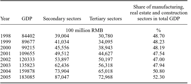
China, as one of the fastest growing economies in the world, is currently in the middle of its drive to industrialize and urbanize. From 1995 to 2005, the share of GDP for the manufacturing and construction industry (known as the secondary sectors) in total GDP rose from 39.9% to 47.5%, while at the same time the official urbanization rate (the share of urban population in total population) rose from 29% to 43.5% (NBS 2006).
Since the mid-1990s, fast industrialization and urbanization in China have been largely investment-driven. Although factors other than capital accumulation were important determinants of GDP growth during the early reform years between 1979 and 1995, during which total factor productivity (TFP) growth accounted for 30% to 58% of China’s development (World Bank 1997; Maddison 1998), the relative contribution of TFP growth to GDP growth declined quickly after the
∗Corresponding author. Email: tao.ccap@igsnrr.ac.cn
ISSN: 1354-7860 print / 1469-9648 online
C
2008 Taylor & Francis DOI: 10.1080/13547860802131300 http://www.tandf.co.uk/journals
mid-1990s. This implies that China’s annual growth above 9% since that time was largely driven by increased capital investment, which grew at the amazing rate of 12.34% per year (Zhenget al.2006).
Investment-driven industrialization and urbanization inevitably involves the displacement of farmers from land around the cities and from places where indus-tries locate. Indeed, land requisitioning has risen significantly since the mid-1990s in China’s suburban areas, with rapid urban expansion and industrialization, as well as large-scale transportation development (Ho and Lin 2004). Accompanying local governments’ promotion of export-oriented development was the establish-ment of thousands of special developestablish-ment zones or industrial districts (Cartier 2001). Since the early 2000s, ‘zone fever’ emerged in China with an indiscrim-inate reproduction of economic development zones and industrial parks across different parts of the country (Zhai and Xiang 2007). However, the land used for such industrial parks and development zones are mostly expropriated with state-defined compensation packages from farmers in suburban areas.
Land use transformations in the processes of industrialization and urbanization in the past decade have resulted in a significant loss of existing arable land in China, as well as causing tens of millions of farmers to become landless. Each year, about 2 to 3 million farmers lose their land to land acquisition that is associated with urban expansion (Tu 2004; Han 2005). Under China’s current legal framework system, farmers’ collectives that own the rural land must first sell it to the state and it is then up to the government to determine the compensation package for land requisition for the purpose of urbanization. In practice, many local governments expropriate farmers’ land with very low compensation and lease it to industrial and commercial developers. In the process of intensifying regional competition for investment, a ‘race to the bottom’ type of game pushes local governments to offer low-cost land to attract industrial investment in order to boost future GDP and revenue growth.
Although there has been much anecdotal evidence of local land development strategies in the competition for industrial development, there is little literature to analyze the issue of local land finance and how it relates to the investment-driven growth witnessed in China during the past decade, nor is there much empirical evidence to evaluate the impacts of local land development on local fiscal revenue and economic growth. By linking China’s investment-driven growth to local land development strategies and evaluating their fiscal impacts, this paper aims to analyze the political economy of local land finance in China. A better understanding of this issue, we believe, will not only help us to understand the political and fiscal incentives of China’s local governments in land development, but will also have important policy implications for future reforms in China’s land institutions.
The rest of this paper is organized as follows. The next section analyzes the important role played by Chinese local governments in promoting industrial de-velopment and how such roles relate to the investment-driven growth witnessed in China. The third section analyzes the institutional background of local land
finance by arguing that one of the key instruments employed by local govern-ments in regional investment competition is to provide cheap land for industrial investors. On the basis of a panel data of China’s provinces from 1995 to 2005, the fourth section examines the simultaneous and lagging impacts of land leasing on local budget revenue and GDP growth. The final section concludes with policy implications.
Local development strategies and investment-driven growth in China
Decentralization and local development state
As China experiences a transition from a centrally planned economy to an increas-ingly market-driven economy in the past two and a half decades, the forces of decentralization, marketization and political legitimization have transformed the country’s local governments into local states with a strong interest in economic de-velopment. Under China’s current political regime, the political legitimacy of the state largely builds on its ability to deliver economic growth and employment. This is why the Chinese government started its market-based reform in the late 1970s and the early 1980s after the chaos of the Cultural Revolution. Under the strategy of ‘Reform and Opening up’, the Communist Party of China has been advocating the objective of catching up with the developed countries, and so high GDP growth has been included in the central government’s policy agenda for decades. Accord-ingly, local governments in the reform period of China have behaved essentially like a developmental state that is strongly motivated to realize economic progress (Oi 1999). As some scholars have observed (Qian and Weingast 1996; Zhu 2004), all layers of government have strong incentives to push their subordinate levels toward output and revenue growth.
Decentralization, both administrative and fiscal, has played a large role in shaping local governments’ behavior during the reform period. The economic reforms initiated since the late 1970s can be characterized as a process of delegating more decision-making powers to the local level, which in turn pushes toward local innovative policies that may gradually lead to marketization (Montinolaet al. 1995; Qian and Weingast 1996). From the administrative perspective, the role of local governments in investment approval, entry regulation, and resource allocation has been significantly enhanced. Beginning in the early 1980s and continuing through the 1990s, there was also the delegation of more state-owned enterprises to local governments at the provincial, municipality, and county levels.
The fiscal dimension of decentralization was no less dramatic. In 1980, the inter-governmental monetary system shifted away from ‘unified administration of revenue and expenditures’ toward ‘cooking in separate kitchens’ (fenzao chi-fan), which divided revenue and expenditure responsibilities between the central and the provincial governments (Qian 1999, 2000; Wong 2000). After that, the central-provincial fiscal arrangement experienced further changes, such as the proportional-sharing system in 1982 and the fiscal-contracting system in 1988. In the 1988 fiscal-contracting system, the central government negotiated different
contracts with each province on revenue remittances to the state and permitted most provincial governments to retain the bulk of new revenues.
All the administrative and fiscal decentralization measures have provided lo-cal governments in China with strong incentives to promote economic growth and mobilize revenue in their jurisdictions. The positive roles of decentralization have been emphasized by some economists who advocate the ‘second generation fed-eralism’. It is argued that the ‘market-preserving federalism’ witnessed in China has been a key factor in China’s growth miracle in the reform period (Montinola et al. 1995; Qian and Weingast 1997). Therefore, by devolving regulatory author-ity from the c