BioSystems 58 (2000) 239 – 247
Emergence of oscillations in a model of weakly coupled two
Bonhoeffer – van der Pol equations
Yoshiyuki Asai *, Taishin Nomura, Shunsuke Sato
Graduate School of Engineering Science,Osaka Uni6ersity,1–3,Machikaneyama,Toyonaka,Osaka560-8531,Japan
Abstract
Bifurcations of periodic solutions in a model of weakly coupled two Bonhoeffer – van der Pol equations are studied. The model realizes a half-center model with reciprocal inhibition, a typical model used in the field of neural motor control to account for the generation of alternating rhythmic bursts observed in motoneurons and spinal neural networks. Several oscillatory solutions such as in-phase, anti-phase as well as out-of-phase solutions emerge from the model’s equilibrium as one of the parameters of the model changes. Among the variety of bifurcations exhibited by the model, we analyze Hopf bifurcations, by which several periodic solutions emerge, and illustrate generation mechanisms of alternating oscillations in the model. © 2000 Elsevier Science Ireland Ltd. All rights reserved.
Keywords:Coupled oscillator; Hopf bifurcation; Reciprocal inhibition
www.elsevier.com/locate/biosystems
1. Introduction
In the study of motor control, alternating bursts of motoneurons and spinal interneurons provide a basis of coordinated limb movements. They involve discharges of motoneurons innervat-ing antagonist muscles, i.e. the extensor and flexor muscles, as well as those controlling muscles of left and right limbs. The generation mechanism of the alternating bursts has been understood in terms of half-center models whose foundation, in many cases, is associated with reciprocal inhibi-tion (Getting, 1981; Grillner et al., 1983). Each half-center has been modeled by an oscillator,
which represents activity of a population of neu-rons or a single neuronal membrane, and the two half-centers are connected mutually by reciprocal inhibition. It is expected that when one center is active, the other is silent, and vice versa. In this way, certain symmetry between the two half-cen-ters is introduced in the models. Symmetrically coupled oscillators modeling the neural genera-tion of walking rhythms can be considered as natural extensions of half-center models.
Several studies have examined generation of the walking patterns by analyzing the dynamics of ordinary differential equations for symmetrically coupled oscillators (Kimura et al., 1993; Taga, 1995). In these studies, parameters of the models such as coupling strengths were determined em-pirically so that the model can reproduce alternat-ing and coordinated patterns observed in animal
* Corresponding author. Tel.:+81-6-68506534; fax:+ 81-6-68506557.
E-mail address:[email protected] (Y. Asai).
Y.Asai et al./BioSystems58 (2000) 239 – 247 241
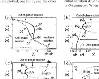
mensional subspace at the left side sH as z in-creases, and a stable periodic solution bifurcates from the equilibrium. It shows in-phase oscilla-tion, i.e. two BVPs oscillates synchronously. Asz
increases further, the equilibrium becomes un-stable in another two-dimensional subspace at the right side sH, and an unstable anti-phase periodic oscillation (two BVPs oscillate with phase-shifted by a half of the oscillation period) bifurcates from the equilibrium. Another stable periodic oscilla-tion branch bifurcates from the in-phase branch (after passing through two pds). It shows out-of-phase oscillation, i.e. two BVPs oscillate with neither in-phase nor anti-phase, and oscillation amplitudes of x1 and x2 are different. For this
reason, two branches bifurcating from the in-phase branch are plotted; one forx1and the other
for x2.
It is important to note that the aforementioned two Hopf points, if they exist, coincide when
d=0 in Eq. (1) regardless of the value ofe. This means that Hopf bifurcations in the model with
d=0 is degenerate, and non-zerodcan unfold the degeneracy. In the singularity theoretic bifurca-tion analysis (Golubitsky and Schaeffer, 1985), an appropriate singularity is chosen for a given bifur-cation problem, and bifurbifur-cation structure of the model is analyzed in the vicinity of the singularity. We will chose the case d=0 ande=0 in Eq. (1) as the highest singularity for our analysis.
Our analysis depends fully on the symmetry of the system. If a mapping f(x) commutes with a group G, i.e. ÖgG, f(g·x)=g·f(x), we say that
f(x) isG-symmetry. Similarly, an ordinary differ-ential equation dx/dt=f(x) isG-symmetry iff(x) is G-symmetry. When e=0 andd=0 in Eq. (1),
two BVPs are independent, i.e. there is no interac-tion between two BVPs. Thus, Eq. (1) commutes with group actions that cause the phase-shift of the periodic solution of each BVP independently. Due to this symmetry, in the case of e=0 and
d=0, Eq. (1) can be reduced to the mapping, which commutes with Z2Z2 (see Section 3 for
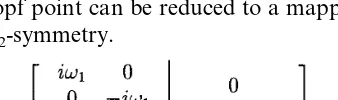
definition). According to Golubitsky et al. (1988), in addition, a Birkhoff normal form of a given system whose linear part has the following form at a Hopf point can be reduced to a mapping with
Z2Z2-symmetry.
(2)
where 9iv1 and 9iv2 are two distinct pairs of
complex conjugate purely imaginary eigenvalues. Since the linear part of Eq. (1) withd=0 at Hopf point has the form of Eq. (2), it is expected strongly that Eq. (1) may exhibit bifurcations similar to those for systems in Birkhoff normal form with linear part as in Eq. (2).
The bifurcation problem of Z2Z2-symmetry
mappings (i.e. finding the zeros of algebraic equa-tions as a function of a bifurcation parameter and their qualitative changes when auxiliary parame-ters change) has been studied by Golubitsky and Schaeffer (1985). In this paper, we analyze the bifurcation of periodic solutions in Eq. (1) in relation to that of the mapping with Z2Z2
-symmetry.
3. Bifurcation problem with Z2Z2 symmetry
In this section, we summarize the bifurcation problem of a Z2Z2-symmetry mapping with
two state variables. This is necessary for our analysis below. Z2Z2 acting on R
try mapping with two state variables, where lis a bifurcation parameter. The bifurcation problem
g=0 has four solution types — (a) trivial solu-tion, x=0, y=0, (b) x-mode solution, x"0,
y=0; (c) y-mode solution, x=0, y"0; and (d) mixed mode solution, x,y"0. These correspond to the above classification of the points on R2by
their symmetry. By comparing the symmetry of each solution type of Eq. (1) with that of the
Z2Z2-symmetry mapping, it can be seen that
the equilibrium point of Eq. (1) corresponds to the trivial solution. Similarly, the in-phase, anti-phase and out-of-anti-phase solutions correspond to the x-mode, y-mode and mixed mode solutions, respectively. Based on this fact, we associate the bifurcations of periodic solutions in Eq. (1) with those of equilibria in the Z2Z2-symmetry
map-ping. Consider the following Z2Z2-symmetry
normal form h given by
h(x,y,l)=
(e1xreal numbers. We assume that h satisfies the fol-lowing non-degeneracy conditions,
m"e2e3e4, n"e1e2e4, mn"e1e3. (4)
Among the six coefficients inh, let us fixei(i=
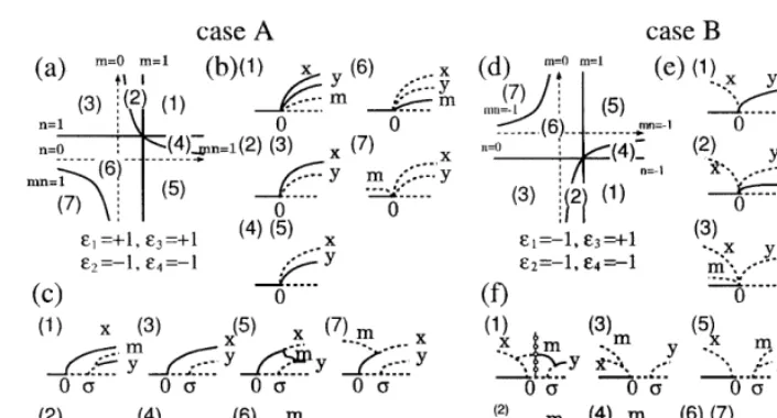
1,2,3,4) for a moment. The BD ofhis obtained by plotting solutions of h=0 as a function of the bifurcation parameter l. The form of the BD changes as m and n change. The non-degeneracy conditions in Eq. (4) divide the m–n plane for a given set of ei(i=1,2,3,4) into several regions as
shown in Fig. 2(a) and (d). BDs are topologically equivalent for all values of m and n within each region. Now, for another set ofei(i=1,2,3,4), we
have a different m–n plane, which is also divided into several regions. There are 16 possible combi-nations of signs e1, e2, e3 and e4. Let us
concen-trate on case A (Fig. 2(a – c), e1=e3= +1,
Y.Asai et al./BioSystems58 (2000) 239 – 247 243
Fig. 2. Examples of BD for case A ((a), (b) and (c)) — e1=e3= +1,e2=e4= −1, and for case B ((d), (e) and (f)):e3= +1, e1=e2=e4= −1. (a) and (d) — Then–mplanes. The solid curves represent the non-degeneracy conditions. (b) and (e) — BDs ofh=0 with respect tol. (c) and (e) — Perturbed BDs, i.e.s"0, with respect tol. In (b), (c), (e) and (f), the solid and dashed curves represent stable and unstable solutions, respectively. Symbolsx,y, andmstand for ax-mode,y-mode and a mixed mode solutions, respectively. Numbers in (b) and (c), and in (e) and (c) correspond to those attached to the regions in (a) and (d), respectively. In (f), the branches indicated by open circles represent periodic solutions, which we do not investigate in details in this paper.
number.h has a unique bifurcation pointl=0 at whichx-mode,y-mode and mixed mode solutions emerge from the trivial solution simultaneously (no mixed mode solutions emerge in Fig. 2(b)-(2,3,4,5)). In this sense, this bifurcation point is a singularity of h=0. The linearized stability of each solution is determined by the eigenvalues of the Jacobian matrix, and it is invariant under equivalence as far as the non-degeneracy condi-tions are satisfied. Thus, the BDs of the normal form h and those of other mapping, which is
Z2Z2-equivalent to h have one-to-one
correspondence.
Small perturbation terms added to h can change qualitatively the form of the BD of h=0, i.e. the normal form is structurally unstable, and we have perturbed BDs. Such perturbations may unfold the singularity ofh. All possible changes in the form of BDs of perturbed h can be analyzed by looking at the BDs of a universal unfoldingH
of h, which is Z2Z2-equivalent to any
unfold-ings ofh.
H(x,y,l,a)=
(e1x2+m˜ y2+e 2l)x
(n˜x2+e
3y2+e4(l−s))y
(5)where (m˜,n˜,s) varies on a neighborhood of (m,n,0). Note that, for a perturbed hwith a given
m and n, we cannot specify the values of m˜,n˜ in the universal unfolding H explicitly, although the point (m˜,n˜) are close to (m,n) in h. In the case
s"0, H has two bifurcation points l=0 and
l=sfrom which an x-mode and a y-mode solu-tions emerge, respectively. For example, the BD of h with m and n in region (1) of Fig. 2(a) is illustrated in Fig. 2(b)-(1), and its form changes into the perturbed BD as illustrated in Fig. 2(c)-(1). In this case, a stable mixed mode solution bifurcates from the unstable y-mode solution. Note that both the coupling constant din Eq. (1) and the unfolding parameter s in Eq. (5) unfold the singular bifurcation to less singular bifurcations.
4. The reduction
sys-tem can be reduced by Liapunov – Schmidt method to a mapping with one state variable. The reduced mapping is equivalent to a pitchfork bifurcation. Zeros of the reduced mapping are locally in one-to-one correspondence with orbits of small amplitude periodic solutions to the system. Thus, bifurcation analysis of the reduced mapping can reveal the bifurcation of a periodic solution branch in the original system.
When two Hopf points coincide (a double Hopf) in our model Eq. (1) with d=0, the theorem cannot be applied. To analyze onsets of periodic solutions by a double Hopf in Eq. (1), we reduce Eq. (1) with this singularity to a mapping with two state variables for the coupling constants
e small enough and d=0. The mapping is
Z2Z2-equivalent to the normal form h defined
in the Section 3. From the equivalence, we can calculate the coefficients of h such as ei
(i=1,2,3,4), m and n, once the parameter values of Eq. (1) such as b and care specified. Detailed calculation is omitted here, and will be described elsewhere.
It is important for our analysis to mention that we assumed that Eq. (1) with no couplings (the uncoupled two BVPs) can be considered as the singular point of the coupled BVPs, from which several less singular bifurcation problems are unfolded for non-zero small coupling constants e
and d. When e=d=0, the two identical BVPs are uncoupled, and two Hopf bifurcations (one for each BVP) occur simultaneously. This can be considered as a special case of double Hopf bifurcation. A periodic solution emerging via one Hopf is the same as another one via another Hopf in terms of their periods, amplitudes and directions of the solution branches on the BD. The two periodic solutions, however, can show arbitrary phase differences. We consider the coupling constants d, as well as e, as perturbations to the bifurcation problem of the uncoupled BVPs. It can be shown that the singularity with the double Hopf is persistent against the perturbation by the coupling o
imposed to the uncoupled BVPs, but phase differences between two periodic solutions are restricted by the perturbation to particular phase differences (such as in-phase, anti-phase, and
out-of-phase). In this sense, e unfolds the singularity in the uncoupled BVPs. When the singularity is unfolded by d, the two Hopf points become distinct, and the corresponding BDs can be analyzed in comparison to those of the universal unfolding of the reduced mapping.
5. Hopf bifurcations in the coupled BVP equations
First, we illustrate BDs of the uncoupled BVPs (e=d=0) for the reason mentioned in the previ-ous section. Each of the two identical Hopf bifur-cations can be reduced to a scalar mapping describing a pitchfork bifurcation. Bifurcation analysis of the scalar mapping tells us the direc-tions and stabilities of periodic solution branches in each single BVP. The b–c parameter plane of Eq. (1) can be divided into several regions as shown in Fig. 3(a). Within each region, the BDs are equivalent. In region 1, two periodic solution branches are supercritical and neutral stable for any phase difference (dot-dashed curves). Note that only one branch in each BD of Fig. 3(a) is depicted since the two periodic solution branches are identical. In regions 2 and 3, they are subcrit-ical and unstable (dashed curves). Fig. 3(b) shows theb–cplane for non-zero smalleandd=0. This can be obtained from detailed analysis of a re-duced mapping with two variables. Comparison of Fig. 3(a) and (b) reveals influences of the coupling by e on the form of the BD, i.e. in-phase, anti-in-phase, and out-of-phase (mixed mode) solutions appear.
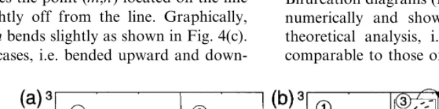
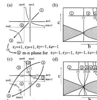
Fig. 4 illustrates changes in the form of the BD as the parameter b (andc) changes. We examine correspondences between Fig. 4(a) and (b). The BDs for regions labeled by the same numbers in Fig. 4(a) and (b) are the same. Note that the BDs of the normal formh for each region in Fig. 4(a) are illustrated in Fig. 2(b). The trace in the b–c
plane (the long arrow in Fig. 4(b)) and those in the coefficients ofh such asei(i=1,2,3,4), mand
n (the set of arrows in Fig. 4(a)) are compared. When the point (b,c) in theb–cplane is located in region 1 of Fig. 4(b), the set of calculated coeffi-cients ofh(the point (m,n) withe1=e3= +1 and
Y.Asai et al./BioSystems58 (2000) 239 – 247 245
4(a). Region boundaries in Fig. 4(a) and (b) are also numbered with the parentheses, and the boundaries labeled by the same numbers imply that they represent the same change in the form of the BD taking place at the boundaries. When the point (m,n) moves across the boundary (1), which is the point in this case, in Fig. 4(a) (for example), the point (b,c) also moves across the boundary (1) in Fig. 4(b). Let us consider the case that a given point (b,c) moves along the arrow in Fig. 4(b). Then the point (m,n) moves along the arrows (the linem=n and others) in Fig. 4(a). The boundary (3) corresponds to the change of signs ofo1ando3,
and the point (m,n) moves from the m–n plane for e1=e3= +1 and e2=e4= −1 to that for
e1=e3= −1 and e2=e4= −1.
Fig. 4(c) and (d) illustrate the case when the double Hopf singularity is unfolded into two dis-tinct bifurcation points by perturbations in d in the coupled BVPs. In a similar way as Fig. 4(a) and (b), the trace in the b–c plane is compared with that in the parameter space of coefficients in the universal unfoldingH. In the singularity theo-retic approach, the coefficientsoi and (m˜,n˜) inH
are close to those of unperturbed h under small perturbation ind. Remember that the point (m,n) moves along the line m=n in the unperturbed h
as the parameterb(andc) changes. The perturba-tion indforces the point (m,n) located on the line to move slightly off from the line. Graphically, the linem=nbends slightly as shown in Fig. 4(c). Two typical cases, i.e. bended upward and
down-ward, are shown. Thus, as the point (b,c) moves along the arrow in Fig. 4(d), the point (m˜,n˜) moving along the bended curve can visit new regions to which them=ndoes not overlap in the case d=0. Since the six different regions are accumulated at the boundary (1) (m=n=1) in Fig. 4(a), the new regions appear near the boundary (1) in Fig. 4(b). These new regions are illustrated as regions 2 and 3 in Fig. 4(d). Corre-sponding BDs can be seen in Fig. 2(c). Because the boundary (2) in Fig. 4(a) and the line m=n
intersect generically, no new regions appear near the boundary by the perturbation as shown in Fig. 4(c). Another new region appears in associa-tion with the changes of signs ofe1 ande3. When
the point (m˜,n˜) moves across the boundary (5) in Fig. 4(c), only the sign ofe1flips from +1 to −1 and that of e3 remains at +1, leading to a situation illustrated in Fig. 2 case B, and region N in Fig. 4(d) emerges. Then at the boundary (6) in Fig. 4(c), the sign of e3 flips to −1.
6. Discussion
We investigated the bifurcations in the weakly coupled two BVPs in relation to the bifurcations of equilibria of the Z2Z2-symmetry mapping.
Bifurcation diagrams (BDs) of the model obtained numerically and shown in Fig. 1 support our theoretical analysis, i.e. the BDs in Fig. 1 are comparable to those of the universal unfolding H
Fig. 4. Them– n plane and theb–c plane. (a) The n–mplane for e1=e3= +1,e2=e4= −1 for the normal formh. (b) The schematicb–c plane for non-zeroo andd=0. (c) Then–mplane fore1=e3= +1, e2=e4= −1 and parameter traces for the universal unfolding. (d) Theb–cplane for non-zeroeandd. The regions labeled by the same numbers with open circles in (a) and (b) and (c) and (d) are accompanied by the same bifurcation diagrams. The numbers with parentheses indicate the corresponding boundaries. Arrows indicate traces of the points (b,c) in (b) and (d) and of the points (m,n) in (a) and (c). Bifurcation structure in the meshed oval regions have not been well understood.
(Fig. 1(c) and (f) and others not shown in this paper). In this section, we summarize the com-parison to illustrate generation mechanisms of alternating oscillations in the model.
Fig. 1(a) is the BD for a=0.7, b= −0.28,
c=2.0, e=0.01 and d=0.01. It shows two dis-tinct supercritical Hopfs and the out-of-phase branch emerges from the anti-phase branch. Note that the two Hopfs are supercritical by the change of stability as the bifurcation parameter moves across the Hopf point from left to right in the figure, although the two periodic solution
Y.Asai et al./BioSystems58 (2000) 239 – 247 247
far from the Hopf point. Thus, the emergence of this out-of-phase solution may be outside the framework of the singularity theory, and this may cause the difference. In order to take into account the double-cycle bifurcations and the emergence of the out-of-phase solution in this case, we need to choose another normal form, which contains higher order terms such asx5,xy4forhin Section
3, and to consider the higher singularity of the system.
The BD in Fig. 1(b) and that of in Fig. 2(c)-(6) are compared. From the correspondence, the point (b,c)=(0.53,2.0) may be located in region 4 of Fig. 4(d). They are equivalent in the type of Hopf bifurcations and the emergence of the out-of-phase branch including its stability. One differ-ence is that the out-of-phase branch bifurcating from the in-phase branch has the double-cycle bifurcations and connects to the anti-phase branch in Fig. 1(b), whereas the mixed mode branch emerging from the x-mode branch does not connect to they-mode branch in Fig. 2(c)-(6). This may also be managed by the higher singular-ity of the system. As the parameter b increases from 0.53 to 0.58, the supercritical Hopf by which the in-phase solution emerges changes into sub-critical, but the Hopf bifurcation which generates the anti-phase solution remains supercritical. Thus Fig. 1(c) may correspond to Fig. 2(f)-(3), and the point (b,c)=(0.58,2.0) may be located in region N of Fig. 4(d).
Fig. 1(d) includes two subcritical Hopfs. It cor-responds to the universal unfolding H with e1=
e2=e3=e4= −1. Thus the point (b,c)=(1.3,2.0)
may be in region 6 of Fig. 4(d) which is on the
m–n plane for e1=e2=e3=e4= −1. The
bifur-cation structure near the points labeled by uHs in Fig. 1(d) is complicated. It includes global bifur-cations and multiple equilibrium. A Hopf bifurca-tion can take place on every equilibrium among coexisting equilibria, and a periodic solution gen-erated from one equilibrium collides with the other equilibrium. This situation is difficult to study analytically. A detailed numerical analysis is powerful for this case. For example, Kitajima et al. (1998) calculated numerically the detailed BDs of periodic solutions and those of the equilibria in a system of coupled BVP oscillators.
The comparison in the BDs between the re-duced mapping and the coupled BVPs seems to be able to account for the emergence of the in-phase, anti-phase and out-of-phase oscillations in our model as a half-center model with reciprocal inhi-bition. Further analysis should be done, however, to elucidate the conditions for the model to ex-hibit stable anti-phase as well as other coordi-nated oscillations.
References
Collins, J.J., Stewart, I., 1993. Coupled nonlinear oscillators and the symmetries of animal gates. J. Nonlinear Sci. 3, 349 – 392. Ermentrout, G.B., 2000. http://www2.pitt.edu/phase/
Fitzhugh, R., 1961. Impulses and physiological states in theoret-ical models of nerve membrane. Biophys. J. 1, 445 – 466. Getting, P.A., 1981. Mechanisms of pattern generation
under-lying swimming in Tritonia I. Neuronal network formed by monosynaptic connections. J. Neurophysiol. 46, 65 – 79. Golubitsky, M., Schaeffer, D.G., 1985. Singularities and
Groups in Bifurcation Theory I. Springer, New York. Golubitsky, M., Stewart, I., Schaeffer, D.G., 1988. Singularities
and Groups in Bifurcation Theory II. Springer, New York. Golubitsky, M., Stewart, I., Buono, P.L., Collins, J.J., 1999. Symmetry in locomotor central pattern generators and animal gaits. Nature 401, 693 – 695.
Grillner, S., Wallen, P., McClellan, A., Sigvardt, K., Williams, T., Feldman, J., 1983. The neural generation of locomotion in the lamprey: an incomplete account. In: Robert, A, Robert, B (Eds.), Neural Origin of Rhythmic Movements. Cambridge University Press, New York.
Guckenheimer, J., Holmes, P., 1983. Nonlinear oscillations, dynamical systems, and bifurcations of vector fields. Springer, Berlin.
Guckenheimer, J., Rowat, P., 1997. Dynamical systems analyses of real neuronal networks. In: Stein, P.S.G., Grillner, S., Selverston, A.I., Stuart, D.G. (Eds.), Neurons, Networks, and Motor Behavior. MIT Press, Massachusetts, pp. 151 – 163.
Kimura, S., Yano, M., Shimizu, H., 1993. A self-organizing model of walking patterns of insects. Biol. Cybern. 69, 183 – 193.
Kitajima, H., Katsuta, Y., Kawakami, H., 1998. Bifurcations of periodic solutions in a coupled oscillator with voltage ports E81-A. Trans. IEICE E81-A (3), 476 – 482. Marder, E., Kopell, N., Sigvardt, K., 1997. How computation
aids in understanding biological networks. In: Stein, P.S.G., Grillner, S., Selverston, A.I., Stuart, D.G. (Eds.), Neurons, Networks, and Motor Behavior. MIT Press, Massachusetts, pp. 139 – 149.