E-mail address:[email protected] (S.F. Nielsen)
On simulated EM algorithms
Soren Feodor Nielsen
Department of Theoretical Statistics, Institute of Mathematical Sciences, University of Copenhagen, Universitetsparken 5, 2100 Kopenhagen 0, Denmark
Received 1 August 1997; received in revised form 1 May 1999
Abstract
The EM algorithm is a popular and useful algorithm for "nding the maximum likelihood estimator in incomplete data problems. Each iteration of the algorithm consists of two simple steps: an E-step, in which a conditional expectation is calculated, and an M-step, where the expectation is maximized. In some problems, however, the EM algorithm cannot be applied since the conditional expectation required in the E-step cannot be calculated. Instead the expectation may be estimated by simulation. We call this a simulated EM algorithm. The simulations can, at least in principle, be done in two ways. Either new independent random variables are drawn in each iteration, or the same uniforms are re-used in each iteration. In this paper the properties of these two versions of the simulated EM algorithm are discussed and compared. ( 2000 Elsevier Science S.A. All rights reserved.
Keywords: Simulation; EM algorithm; Incomplete data
1. Simulated EM algorithms
The EM algorithm (cf. Dempster et al., 1977) has two steps, an E-step and an M-step. The E-step is the calculation of the conditional expectation of the complete data log-likelihood given the observed data. The M-step is a maximi-zation of this expression. These two steps are then iterated. Each iteration of the algorithm increases the observed data log-likelihood, and though the general
convergence theory is rather vague, the algorithm often works well in practice. Ruud (1991) gives an overview of the general theory and some applications to econometrics. For more on the EM algorithm, see McLachlan and Krishnan (1997).
However in some cases the E-step of the algorithm is not practically feasible, because the conditional expectation cannot be calculated. This happens for instance when the expectation is a large sum or when the expectation corres-ponds to a high-dimensional integral without a closed-form expression. In this case, the expectation could be replaced by an estimate obtained by simulation. We shall call the resulting algorithm a simulated EM algorithm, a name taken from a paper by Ruud (1991). More or less di!erent ways of constructing this estimate have been suggested by Celeux and Diebolt (1985), Wei and Tanner (1990), and McFadden and Ruud (1994). The di!erence between these ideas are discussed below after a more formal de"nition of the simulated EM algorithm.
LetX
In the M-step this function is maximized overh, and the maximizer is then used as a new value of h@ in the subsequent iteration. In this way we get a sequence ofh-values,h
1, h2,2say, which converge under weak assumptions to
the local maximizer (cf. Wu, 1983).
One iteration of the EM algorithm thus corresponds to calculating the conditional expectation (1) and maximizing it as a function of h. We denote the EM update, i.e. the h-value given by one iteration of the EM algorithm starting inh@, byM(h@). The maximum likelihood estimator,hKn, is a"xed point of
M, i.e. a solution toM(h)"h. The EM algorithm"nds"xed points ofMby the method of successive substitution; from a starting value,h1, ofh,h2"M(h1) is calculated and used to calculateh3"M(h2), etc.
In the simulated EM algorithm the expectation (1) is replaced by an estimate in the following way: LetXI ijforj"1,2,mbe a random variable drawn from the conditional distribution ofX
is an unbiased estimate ofQ(hDh@). In practice,XI ijis simulated using one or more uniform (pseudo-) random numbers. ThusXI ij"g(;
ijD>i, h@) for some function
g()Dy, h), where the;ij's are independent (vectors of) uniform random variables,
independent of the>
uniform random variables, depends on the dimension of theX
i's as well as on
the method of generating the XIij's. We shall not go further into the actual generation of theXIij's, since all that matters for the results of this paper is the fact that the simulations are based on a sequence of (pseudo-) random numbers; they need not even be uniform, but generally they are.
We get two fundamentally di!erent simulated EM algorithms according to whether we draw new independent random variables in each iteration or we re-use the uniforms,;
ij, in each iteration.
Drawing new uniforms in each iteration, the sequence of h-values obtained from the algorithm, (hI
n(k))k|N, is a Markov chain, which is typically ergodic. As
kPR, the distribution ofhI
n(k) approaches the stationary initial distribution of
the Markov chain. The estimator obtained, when the algorithm has converged, is thus a random variable drawn from the stationary initial distribution of the chain. This version has been discussed in detail by Nielsen (2000). It is essentially
the &stochastic EM algorithm' suggested by Celeux and Diebolt (1985) (see
Diebolt and Ip, 1996 for a review), which also uses new uniforms in each step of the algorithm but only allowm"1.
Reusing the uniforms, we estimate the functionhPM(h) once and for all and search for "xed points of the estimated function by the method of successive substitutions. Since a"xed point,h@, ofMhas 0"DhQ(hDh@)@h/h{, this essentially corresponds to "nding a root of
G
This is done by the method of successive substitutions: Starting with a given value ofh@, the next value is found by"nding the root of
D
which is then used to"nd the next value, etc. In practice of course there may well be more than one root of DhQI(hDh@); the root we need to pick is the one maximizingQI(hDh@). Notice thatG
n(h@) is an unbiased estimate ofDhQ(hDh@)@h/h{if
di!erentiation and expectation are interchangeable. This version is discussed by McFadden and Ruud (1994) as a special case of the method of simulated moments.
So we have two versions of the simulated EM algorithm; in one we keep drawing new random numbers (leading to a Markov chain ofh-values), and one in which we re-use the uniforms.
re-used, theSimEMalgorithm. One should note that in the literature the acro-nym SEM is used by McFadden and Ruud (1994) for the SimEM algorithm, but it is also the commonly used acronym for the stochastic EM algorithm sug-gested by Celeux and Diebolt (1985). For this reason we avoid the acronym SEM. Also the supplementary EM algorithm (cf. Meng and Rubin, 1991), which is not a simulated EM algorithm, is denoted SEM in the literature.
It should be clear that at least for moderate values ofmthe two versions di!er signi"cantly. The purpose of this paper is to compare these two simulated EM algorithms.
As noted above StEM is essentially just the stochastic EM algorithm sugges-ted by Celeux and Diebolt (1985). The only di!erence is that we here allow
m'1. Diebolt and Celeux (1993) discuss estimation of mixing proportions using the stochastic EM algorithm and give some asymptotic results for this case. Nielsen (2000) gives asymptotic results under general smoothness assump-tions.
It is not clearly stated by Ruud (1991) which version of the simulated EM algorithm he considers. However, the suggested asymptotic results and the paper by McFadden and Ruud (1994) indicates that it is the SimEM version rather than the StEM version, he has in mind. However, his de"nition would allow StEM as well as SimEM as a simulated EM algorithm, and we therefore use the termsimulated EM algorithmto denote both StEM and SimEM.
Wei and Tanner (1990) suggest to calculate the conditional expectation needed in the E-step of the EM algorithm by Monte Carlo integration, leading to the so-called MCEM algorithm. With our notation this corresponds to
m"R. In this case it does not matter whether we re-use uniforms or draw new uniforms in each iteration. In practice, of course, m(R and the results discussed in this paper thus also applies to the MCEM algorithm. Ignoring that
m(Rwill lead to underestimation of the asymptotic variance of the estimator, since we then ignore the noise added by the simulations.
Other ways of using simulation in estimation exist. One method is the method of Monte Carlo likelihood, where we attempt to estimate the observed data log-likelihood function using simulation and then maximize this estimated function (see Geyer, 1996 for a recent review). A closely related method is the method of simulated scores (MSS) suggested by Hajivassiliou and McFadden (1997). Another possibility is to specify a Bayesian model and use Gibbs sampling or other MCMC methods to estimate the parameters. These methods are discussed further in Section 6.
2. Asymptotic results
We begin this section by introducing some notation. All score functions
Letf
h be the density ofX. Letsx(h) be the corresponding score function and
put<(h)"E
h(sX(h)sX(h)5); the superscript t denotes transpose. Leth0denote the
true unknown value ofh3H-Rd.
The score function corresponding to the conditional distribution ofXgiven
>"ywith densityxPgh(xDy) is denoteds
x@y(h). LetIy(h)"Eh(sX@y(h)sX@y(h)5D>"y).
Lets
y(h) be the score function corresponding to the distribution of>and put
I(h)"Eh(s
meterhis locally identi"ed from the complete data as well as from the incom-plete data. Of course this is necessary in order to estimate the parameter.
Finally we putF(h)"E
hIY(h)<(h)~1. This can be interpreted as the expected
fraction of missing information (cf. Dempster et al., 1977). We will need the following facts aboutF(h):
Lemma 1. The eigenvalues ofF(h0) are real, non-negative, and smaller than 1.
F(h0)hasdlinearly independent eigenvectors corresponding to thedeigenvalues. The rank ofF(h0)equals the number of non-zero eigenvalues.
Proof. Since <(h
0) is positive-de"nite, it has a positive-de"nite square-root,
<(h
0)1@2. Let<(h0)~1@2be the inverse of this square root.
Since F(h
0) is similar to the positive-semi-de"nite matrix
<(h
0)~1@2F(h0)<(h0)1@2"<(h0)~1@2Eh0IY(h0)<(h0)~1@2, it has d linearly
inde-pendent eigenvectors and real, non-negative eigenvalues (cf. Lancaster, 1969). Furthermore,F(h
0) has the same rank as this symmetric matrix, which has rank
equal to the number of non-zero eigenvalues.
Ifjis an eigenvalue andethe corresponding eigenvector, thenF(h0)e"je,
Asymptotic results for the StEM algorithm were discussed by Nielsen (2000, Theorem 1), who proved the following result under general regularity condi-tions:
Theorem 1 (Asymptotic results for the StEM algorithm). If the Markovchain is ergodic and tight,thenJn(hI
Remark. Ergodicity and tightness can be checked as in Nielsen (2000).
Recall thathInis a random variable drawn from the stationary initial distribu-tion of the Markov chain constructed in the StEM algorithm. The theorem states that the stationary distribution of the Markov chain converges weakly to a normal distribution as the sample size increases.
We shall not give a detailed proof of Theorem 1 here; see Nielsen (2000) for a precise statement of the regularity conditions as well as a general proof of the result. We will however give a proof for the case of exponential family models, which includes many models of practical interest as noted by Ruud (1991). Since this proof is rather long, it is deferred to the appendix. Example 1 in the following section proves this theorem and Theorem 2 below in a special case with Gaussian distributions, where the results hold exactly and not only asymptotically.
In order to obtain asymptotic results for the SimEM version, we apply Corollary 3.2 and Theorem 3.3 in Pakes and Pollard (1989). McFadden and Ruud (1994) give similar results under stronger assumptions.
Using Eh
0 to denote expectation under the true distribution of the>i's and
theXI ij's, we note that
G(h)"E
h0(Gn(h))"Eh0(Dhlog fh(XI ij))"Eh0Eh0(Dhlogfh(XI ij)D>i)
"E
h0Eh(sX(h)D>)"Eh0(sY(h)#Eh(sX@Y(h)D>))
"Eh
0(sY(h)).
In the fourth equality note that Eh
0(Dhlogfh(XI ij)D>i)"Eh(sX(h)D>); this is how
the XI ij are simulated. G(h) is di!erentiable under usual regularity conditions with
DhG(h)@h/h
0"I(h0). (4)
Furthermore, by the central limit theorem
JnG
n(h0) D
PN
A
0,I(h0)#1m Eh0IY(h0)
B
. (5)By assumptionG(h0)"0 and we will assume that there is a neighbourhood of
h0such thath0 is the only root ofGinside this neighbourhood.
From the law of large numbers, we know that G
n(h)PP G(h) for all h. This
needs to be extended to uniform convergence to obtain consistency. Also, by the central limit theorem,Jn(G
to be close toJnG
n(h0) whenhis close toh0. To be precise we need these two
assumptions:
(A1) suph|
CDDGn(h)!G(h)DD/(1#DDGn(h)DD#DDG(h)DD)PP 0, for a compact
neigh-bourhood,C, ofh0. (A2)
sup@@h~h
0@@:dn(JnDDGn(h)!G(h)!Gn(h0)DD)/(1#JnDDGn(h)DD#JnDDG(h)DD)
P
P0, for anyd
nP0.
Stronger assumptions are obtained if the numerators are ignored. A su$cient condition for both assumptions is given in this lemma (see Pakes and Pollard, 1989 for weaker conditions):
Lemma 2. Suppose that in a neighbourhood ofh0for somea'0
Dlogfh(g(;D>, h))!logfh{(g(;D>,h@))D)t(;,>)DDh!h@DDa
(i) IfE
h0Dt(;,>)D(Rthen(A1)holds.
(ii) IfEh
0t(;,>)2(Rthen(A2)holds.
Proof. See Lemmas 2.13, 2.8, and 2.17 in Pakes and Pollard (1989). h
We say thathI
nis an asymptotic local minimum ofDDGn(h)DDif for some open set
=-HDDG
n(hIn)DD)infh|WDDGn(h)DD#oP(n~1@2). From Corollary 3.2 and Theorem
3.3 in Pakes and Pollard (1989) we get the following result:
Theorem 2 (Asymptotic results for the SimEM algorithm). Under assumption
(A1),there is an asymptotic local minimum,hIn,ofDDG
n(h)DDsuch thathInPP h0. Under assumption(A2),if hI
n is consistent,then
Jn(hIn!h
0) D
PN(0, I(h0)~1#(1/m)I(h0)~1Eh
0IY(h0)I(h0)~1).
3. A comparison
It is clear that both the SimEM and the StEM version of the simulated EM algorithm approximates the EM algorithm asmtends to in"nity. Both versions lead to estimators with asymptotic variances tending toI(h0)~1asmPR. For
"nite values of m, however, the asymptotic variances di!er.
Recalling that F(h0)"Eh
0IY(h0)<(h0)~1 and <(h0)"I(h0)#Eh0IY(h0) we
"nd (with the usual ordering of positive de"nite matrices) that
I(h0)~1Eh
0IY(h0)I(h0)~1'<(h0)~1Eh0IY(h0)<(h0)~1(I!F(h0)2)~1
Q(I!F(h0)2)<(h
Q<(h0)Eh0IY(h0)~1<(h0)!E
h0IY(h0)'I(h0)Eh0IY(h0)~1I(h0)
QEh0IY(h0)#I(h0)Eh
0IY(h0)~1I(h0)#2I(h0)!Eh0IY(h0)
'I(h
0)Eh0IY(h0)~1I(h0)
Q2I(h0)'0.
In these calculations we have implicitly assumed that Eh
0IY(h0) is non-singular.
If Eh
0IY(h0) is singular, then some of the eigenvalues ofF(h0) are zero (cf. the
proof of Lemma 1). Suppose thatrof thedeigenvalues ofF(h
0) are 0. Then we
can writeF(h
0)"ab5, whereaandb ared]r-matrices of full rank,spanb5" spanF(h
0) andb5ais non-singular. LetaM be a d](d!r)-matrix of full rank
such thata5Ma"0. Then
hP
C
a5Mhb5h
D
(6)is a bijection ofh(cf. Johansen, 1995). Thus (a5Mh, b5h) is a reparameterization of
h. The fraction of missing information for the parametersa5Mhandb5hare
(b5E
h0IY(h0)b)(b5<(h0)b)~1"(b5F(h0)<(h0)b)(b5<(h0)b)~1"b5a,
(a5ME
h0IY(h0)aM)(a5M<(h0)aM)~1"(a5MF(h0)<(h0)aM)(a5M<(h0)aM)~1"0.
The second line means that there is no missing information abouta5Mh, and the asymptotic variance ofa5MhI
nis easily seen (cf. the proof of Theorem 6) to be 0 for
both versions of the simulated EM algorithm. To handle the parameterb5h, note that the missing information aboutb5h,b5Eh
0IY(h0)b, is non-singular, sinceb5ais
non-singular. Thus we can repeat the argument given above for a non-singular E
h0IY(h0) applied to the information matrices corresponding tob5h, leading to
the conclusion that b5h is strictly better estimated using StEM rather than SimEM.
Hence, we have shown the following result:
Theorem 3. The estimator derived from the StEM algorithm has smaller asymptotic
variance than the estimator derived from the SimEM algorithm,when the samevalue of m, i.e. the same number of simulated values per iteration, is used in both algorithms.
This result may seem counterintuitive as new random noise is added in each iteration of the StEM algorithm. The following example o!ers an explanation.
Example 1. Let X
1,X2,2,Xn be iid bivariate random variables, normally distributed with common expectationhand variances 1 and known correlation
o3]!1; 1[. Suppose only the"rst coordinate,X
1i, of eachXi"(X1i,X2i)5is
observed. The observed data MLE,hKn, is just the average of theX
The simulated EM algorithm (with m"1) corresponds to simulating
X
2i from the conditional distribution ofX2i givenX1i and then averaging all
theX
ji's, the observed as well as the simulated. Thus, in the (k#1)th iteration,
we simulateXI 2i"(1!o)hIn(k)#oX
in the SimEM and the StEM case is thus normal with expectation 0 and variance given by the variance of the MLE plus the variance speci"ed above (in (8) and (9), respectively).
It is not di$cult to show directly that the variance of the StEM estimator is smaller than the variance of the SimEM estimator, and we leave these calcu-lations to the reader. Instead, looking at (7), we observe that
Var(Jn(hIn(k#1)!hK
For the StEM version the covariance term is 0, whereas it is positive for the SimEM version. Thus, we see that the variance of the SimEM estimator is larger exactly because&the uniforms are re-used'.
The Markov chain of the StEM algorithm is irreducible under weak assump-tions, and the StEM algorithm does therefore not&get stuck'in a wrong estimate. If it converges, i.e. if the Markov chain is ergodic, the StEM algorithm converges stochastically in the sense that the sequence of distributions of the h-values obtained from the iterations converge in total variation. There is a growing literature on convergence detection for MCMC methods. Many of these methods for detecting convergence (or rather lack of convergence) of MCMC calculations can be used to detect (lack of ) convergence for any Markov chain. Hence, there exist methods which can be applied to ascertain convergence of the StEM algorithm; see Brooks and Roberts (1998) for a review of these methods. The SimEM algorithm is a deterministic algorithm }an application of the method of successive substitutions } searching for a root of the (random) functionG(h). Hence, if it converges, it converges deterministically. There is no apparent reason to believe that G
n(h) only has one root, and the SimEM
algorithm stops when one is found. Thus multiple runs are needed to ensure that the correct root is found. There may even be no root at all as in the following example. Furthermore, the method of successive substitutions is typically slow (requires many iterations), as is well-known in the case of the EM algorithm. Hence, it is not clear which algorithm is faster in practice.
Example 2. Let X
1,X2,2,Xn be iid normally distributed with expectation
0 and variance h. Observe X
i if Xi*0. The SimEM algorithm (with m"1)
corresponds to iterating
hIn(k#1)"1
n
n
+
i/1
(X2i)1MXiw0N#hIn(k))e2i )1MXi:0N)
wheree
i are iid random variables from the standard normal distribution given
that they are negative. We shall assume that at least oneX
i is observed so that
hcan be estimated from the observed data. Of course, asnPRthis happens with probability 1 by the Borel}Cantelli lemma.
If+ni/1e2
i)1MXi:0N*n(which happens with positive}albeit small} probabil-ity), then hIn(k)PR. If +ni/1e2
i )1M
Xi:0N(n then hIn(k) converges to
+ni/1X2
i )1M
Xiw0N/(n!+ni/1e2i )1MXi:0N) which may be arbitrarily far from the maximum likelihood estimator; the MLE is obtained when +ni/1e2
i )1M
Xi:0N "+ni
/11M
Xi:0N.
Using a contraction principle (cf. Letac, 1986), it is not di$cult to show that the Markov chain of the StEM algorithm for this problem is ergodic so that the StEM algorithm converges.
Using (adaptive) rejection sampling or Markov chain Monte Carlo tech-niques, we can generally simulate theXI ij's. However, neither technique will give us simulations suitable for the SimEM version of the simulated EM algorithm, as neither method&re-uses uniforms'even if we start each iteration with the same random seed. This is due to the random number of iterations needed with these methods. Thus, unless we can simulate theXI ij's in a non-iterative manner, the SimEM algorithm is not really implementable. In Section 4 we shall discuss a way of overcoming this problem. Obviously, this problem does not occur for the StEM algorithm.
To summarize, the StEM algorithm has some theoretical advantages com-pared to the SimEM algorithm: The asymptotic variance is smaller, and the algorithm does not get stuck. Notice also that the SimEM algorithm is not always implementable. On the other hand, convergence is more di$cult to detect in the StEM algorithm than in the SimEM algorithm.
4. Importance sampling
Sampling from the exact conditional distribution ofX
i given>i"yimay in
some cases be impossible. As mentioned previously, iterative methods such as (adaptive) rejection sampling and MCMC methods can often be used to over-come this problem in the StEM algorithm but not in the SimEM algorithm since we would then use a random number of uniforms making it impossible to &re-use'the uniforms in each iteration.
Another way of overcoming this problem is to simulate XI
ij from another
distribution, and then weight the complete data log-likelihoods logfh(XI
ij), to
give an unbiased estimate of the expectationQ(hDh@). This is known as impor-tance sampling.
Suppose that instead of drawing XI ij from the conditional distribution of
X
i given>i"yi with parameterh@, we simulateXI ij from a distribution with
density k
h{()Dyi). Assume that kh{(xDyi)'0 whenever the correct conditional
density ofX
i given>i"yi with parameterh@,gh{(xDyi), is positive. Then
1
n
n
+
i/1
1
m
m
+
j/1
logfh(XI
ij)ch{(XI ijDyi) (10)
is an unbiased estimator ofQ(hDh@), whench{()Dyi)"gh{()Dyi)/kh{()Dyi), since
P
logfh(x)ch{(xDyi)kh{(xDyi) dk(x)"
P
log fh(x)gh{(xDyi) dk(x)"Eh{(log fh(X)D>"y
i),
where dk(x) denotes integration wrt the appropriate reference measure. Typi-cally this corresponds to either ordinary integration (i.e. Lebesgue measure), whenX
This suggests that in the simulated EM algorithms discussed so far, we may replace the assumption ofXI ijbeing drawn from the correct conditional distribu-tion by the less restrictive assumpdistribu-tion thatXI ijis drawn from a distribution with a density, which is positive whenever the density of the correct conditional distribution is.
Importance sampling may be useful for other reasons as well. It obviously changes the variance, and it may be used to reduce the variance of the resulting estimator. Also, especially in the SimEM case, there may be a considerable computational gain in simulating from a distribution, which does not depend on
h@. In this case we can in fact simulate once and re-use the simulatedXI
ij's in each
iteration, rather than re-using the uniforms.
It should be noted however that in order to use importance sampling, we must be able to calculate the importance weights c
h{(XI ijDyi), which depend on the
conditional density ofXgiven>"y
i. Thus we will typically need to know this
density, and hence the density of the observed data. There will still be situations, where knowing the observed data likelihood does not help us"nd the observed data maximum likelihood estimator; here a simulated EM algorithm may be useful. In one special case, the conditional density is not needed: If we can choose a density, fHh{(x), on the complete data sample space so that
hh{(y
i)"fHh{(x)/kh{(xDyi) is the correct density of the distribution of the observed
data (withh"h@), then the importance weights are given as
c
We can easily generalize Theorem 2 to give
Theorem 4 (SimEM algorithm with importance sampling). Under assumptions similar to assumptions(A1)and(A2),there is a local asymptotic minimum,hIn,of
The only change to the argument given in Section 2 is that the variance in (5) is replaced byI(h0)#E
Also the proof of Theorem 1 can be generalized. Again it is a variance that is changed; in the proof in the appendix it is the variance in (14), which is replaced by (1/m)<(h)~1E
h0<arh0(sX@Y(h0)ch0(XD>)D>)<(h0)~1. Hence, we"nd
Theorem 5 (StEM algorithm with importance sampling). Assuming ergodicity and tightness as in Theorem 1, Jn(hI!h
0) D
PN(0, RH
m(h0)),where
RH
m(h0)"I(h0)~1#
1
m
=
+
k/0
F(h0)tk<(h
0)~1
E
h0<arh0(sX@Y(h0)ch0(XD>)D>)<(h0)~1F(h0)k.
Having seen that the results concerning the asymptotic distributions general-ize, the obvious question to ask now is whether Theorem 3 can be generalized too. The proof of Theorem 3 does not generalize, since it relies crucially on the relationship between the involved information matrices, a relationship which Eh
0<arh0(sX@Y(h0)ch0(XD>)D>) plays no part in. On the other hand, it is quite
easily shown that no matter which distribution we choose to sample theXI
ij's
from, there are parameters for which the StEM estimators have lower variance than the SimEM estimators:
Theorem 6. Let e be an eigenvector ofF(h0)and consider the estimatorse5hInofe5h derived from the twoversions of the simulated EM algorithm.
Then the estimator derived from the StEM algorithm with importance sampling has smaller asymptotic variance than the estimator derived from the SimEM algorithm with importance sampling, when the same value of m and the same importance sampling distribution is used in both algorithms.
Remark. The choice ofe5hInas an estimator ofe5hre#ects the fact thate5hKnis the MLE of e5h when hKn is the MLE of h. Since the simulated EM algorithms approximate the EM algorithm and thus maximum likelihood estimation,e5hInis the natural choice.
Notice also that the asymptotic variance of e5hI
n is e5asymp<ar(hIn)e, where
asymp<ar(hI
n) is the asymptotic variance given in Theorems 4 and 5, respectively.
In order to show that one of these matrices is smaller (in the usual ordering of positive-de"nite matrices) we have to show the similar ordering ofu5asymp<ar(hI
n)ufor any vectoru, i.e. that the ordering holds in all directions
Proof. Letjbe the eigenvalue corresponding to the eigenvectore. Recall from Lemma 1 that 0)j(1. Clearly (F(h0))ke"jkeand
e5+=
k/0
F(h
0)5k<(h0)~1Eh0<arh0(sX@Y(h0)ch0(XD>)D>)<(h0)~1F(h0)ke
"+=
k/0 jke5<(h
0)~1Eh0<arh0(sX@Y(h0)ch0(XD>)D>)<(h0)~1jke
" 1 1!j2 e5
<(h
0)~1Eh0<arh0(sX@Y(h0)ch0(XD>)D>)<(h0)~1e.
NowI(h0)~1"(I!F(h0)5)~1<(h
0)~1"+=k/0(F(h0)5)k<(h0)~1so that
e5I(h
0)~1Eh0
<ar
h0(sX@Y(h0)ch0(XD
>)D>)I(h
0)~1e
"+=
k/0 jke5<(h
0)~1Eh0<arh0(sX@Y(h0)ch0(XD>)D>)<(h0)~1
=
+
k/0 jke
" 1
(1!j)2 e5<(h0)~1Eh0<arh0(sX@Y(h0)ch0(XD>)D>)<(h0)~1e.
Since 0((1!j)2)1!j2, the required inequality follows. h
Notice that the result holds forj"0, even though it is more interesting when
j'0, in which case the inequality is strict. The case j"0 corresponds to a direction e in which there is no missing information: e5E
h0IY(h0)e"0 and
consequentlye5hIn has asymptotic variance 0 for both algorithms.
The theorem implies that the StEM algorithm yields better estimates than the SimEM algorithm in the directions given by the eigenvectors. Since the eigen-vectors span Rd (cf. Lemma 1), Theorem 6 shows that if we re-parameterize
hP(e5ih)
i/1,2,dwithe1,2,edthe eigenvectors ofF(h0), then each component of this new parameter is estimated better by using StEM than by using SimEM. It is tempting to conjecture that the estimators obtained from the StEM algorithm are better than the SimEM algorithm. We have not found any counter-examples to this conjecture. However, the theorem does not prove this conjecture, since it does not take the covariances betweene5
ihInande5jhIn into account. The theorem
only implies that the estimators obtained from the SimEM algorithm are not better in the usual (partial) ordering of positive-de"nite matrices than the estimators obtained from the StEM algorithm.
5. Monte Carlo experiment
Let normal variates with mean 1 and variance 2. We simulate 50 replications of
X with b"1,o"0.7 and p2"1.51. The parameter p2 is the conditional variance ofX
1given (X2,X3). This parameterization is chosen because it makes
the parameters variation independent and, consequently, the results easier to interpret.
To investigate the behaviour of the two versions of the simulated EM algorithm we have obtained 1000 estimates from each algorithm, for
m"1, 5, 10. To ensure convergence of the StEM algorithms a burn-in of 15,000 iterations has been used. Thegibbsit-software (Raftery and Lewis, 1992), which in spite of the name can be used for checking convergence of any Markov chain, suggests that a much shorter burn-in is su$cient. After burn-in, 1000 iterations have been performed, and these are used in the results reported below.
The complete data MLE does not have a closed form, and the M-step must be performed numerically. We have used the method of scoring with a "xed tolerance.
The simulated E-step involves drawing values of (X
1,X2) given that they are
both negative. This cannot be done in a non-iterative manner, and as mentioned above this means that the SimEM algorithm is not really implementable. As McFadden and Ruud (1994), we have run a Gibbs sampler for 10 cycles to do this simulation in the SimEM version. In the StEM version, this simulation is done by acceptance-rejection sampling.
The distribution of the simulation estimators, hI!h
0, obtained from the
SimEM and the StEM algorithms can be decomposed into a contribution from the simulations and a contribution from the data,hI!hK andhK!h
0, respectively.
The latter}the distribution of the MLE}is a function of the data only and gives no information on how well the two simulation estimators behave. The simula-tion estimators attempt to approximate the maximum likelihood estimator (cf. Example 1), since the simulated EM algorithm approximates the EM algorithm. Therefore, it is the distribution ofhI!hK that is of interest when evaluating the performance of the simulation estimators. Hence, we look at the empirical distribution of the di!erence between the simulation estimators, hI, obtained from the SimEM and the StEM algorithms and the maximum likelihood estimator,hK.
Table 1
Simulation results forbI!bK
b: (bK"1.042) Mean S.D. 25% Median 75%
m"1: StEM !0.0117 0.0196 !0.0249 !0.0115 0.0013
SimEM !0.0798 0.0122 !0.0878 !0.0808 !0.0724
m"5: StEM !0.0635 0.0104 !0.0702 !0.0637 !0.0565
SimEM !0.0798 0.0055 !0.0838 !0.0799 !0.0762
m"10: StEM !0.0118 0.0065 !0.0162 !0.0117 !0.0074
SimEM !0.0797 0.0038 !0.0822 !0.0798 !0.0772
S.D. is the standard deviation, 25% and 75% are the lower and upper quartiles.
Table 2
Simulation results foro8!o(
o: (o("1.101) Mean S.D. 25% Median 75%
m"1: StEM 0.0386 0.0977 !0.0261 0.0417 0.1061
SimEM !0.2122 0.0917 !0.2733 !0.2118 !0.1527
m"5: StEM 0.0276 0.0408 !0.0003 0.0269 0.0553
SimEM !0.2179 0.0393 !0.2444 !0.2168 !0.1908
m"10: StEM 0.0372 0.0318 0.0148 0.0371 0.0595
SimEM !0.2185 0.0277 !0.2361 !0.2180 !0.1996
S.D. is the standard deviation, 25% and 75% are the lower and upper quartiles.
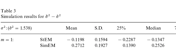
Table 3
Simulation results forp82!p(2
p2: (p(2"1.538) Mean S.D. 25% Median 75%
m"1: StEM !0.1198 0.1594 !0.2287 !0.1347 !0.0291
SimEM 0.2712 0.1927 0.1390 0.2526 0.3787
m"5: StEM !0.1703 0.0623 !0.2112 !0.1750 !0.1324
SimEM 0.2792 0.0836 0.2227 0.2772 0.3318
m"10: StEM !0.1052 0.0523 !0.1424 !0.1066 !0.0712
SimEM 0.2809 0.0584 0.2402 0.2799 0.3216
S.D. is the standard deviation, 25% and 75% are the lower and upper quartiles.
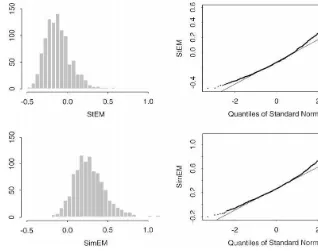
Fig. 1. Histograms and QQ-plots forbI!bK,m"1.
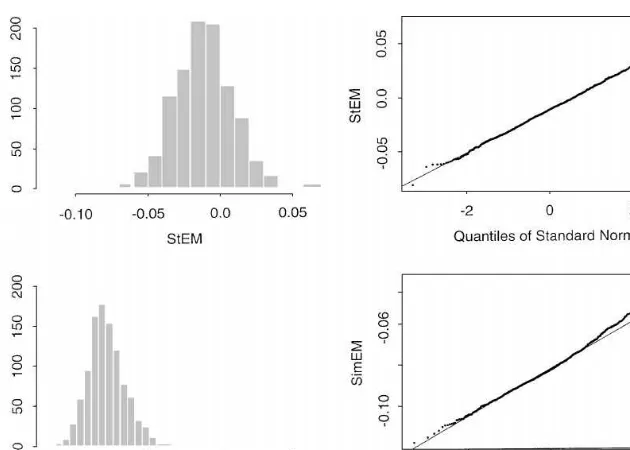
Fig. 3. Histograms and QQ-plots forp82!p(2,m"1.
comparable. The displayed part of the abscissae of the histograms all contain 0, the point corresponding to&no simulation-bias', i.e.hI"hK. Thus, a good method will give a narrow histogram centered at 0. In the QQ-plots a straight line indicates that hI!hK is approximately normal.
Looking "rst at the results for b (Table 1 and Fig. 1) we notice that the variance of the StEM estimator is larger than the variance of the SimEM estimator. This is probably due to the small sample size, as the results of Section 2 indicate that the asymptotic variance is smaller for the StEM estimator.
The bias of the SimEM estimator is however large compared to the bias of the StEM estimator, and the StEM estimator clearly performs better in this example in spite of the larger variance. The fact that the bias of the StEM estimator in the case m"5 is larger than when m"1 or 10 is surprising but also occurs in additional runs of the StEM algorithm for this data (not shown here).
The QQ-plot suggests that both estimators are reasonably close to normally distributed. The tails of the distributions may be a bit too heavy, and the StEM estimator seems to be slightly closer to normal than the SimEM estimator.
We may note that the SimEM estimator is less biased than the StEM estimator when looking at the empirical distribution of o8!o
0 rather than o8!o(. This is due to the large positive bias in the MLE and is thus an e!ect of the data and not the simulations. Consequently, we would not expect the SimEM estimator to perform better than the StEM estimator on all data sets, though itmayperform better wheno( is positively biased. In particular, in large samples, where we would expect the bias of the MLE to be negligible, we would expect the StEM estimator to be superior. Incidentally, this is the only parameter,
h, for whichhI!h
0 is more biased in the StEM case than in the SimEM case.
When estimating p2, the StEM estimator again performs better; the bias is larger for the SimEM estimator, and the variances are here smaller for the StEM estimator.
Fig. 3 shows that the distribution ofp82!p(2is far from normal form"1, but this is what we would expect. Ignoring the multivariate nature of the data and the fact thatp2is not the only parameter, the problem of estimatingp2is very similar to Example 2. Thus, we would expect the SimEM estimator to be distributed approximately as a/(50!s2
12m) for some constantadepending on
the observed data, since only 12X
1's are censored. In particular,p82!p(2is not
approximately normal for small values ofmin the SimEM case. The distribution of the StEM estimator is more di$cult to describe but since the conditional distribution of the next step of the Markov chain in Example 2 given the past is an a$ne transformation of as2
12m-distribution, we would not expectp82!p(2to
be approximately normal for small values of min the StEM case, either. QQ plots for larger values of m (not shown here) shows that the distribution of
p82!p(2gets closer to the normal distribution, whenmincreases. This does not necessarily mean that the distribution of p82!p2 gets closer to normal as
mincreases, sincenis kept"xed.
For all parameters, the standard deviations decrease as m increases. The decrease is roughly 1/J5+0.44 whenmincreases from 1 to 5 and 1/J2+0.71 when going fromm"5 to 10, as we would expect from the asymptotic results. This fact and the distribution of p82!p(2 indicates that as m increases the empirical distribution of the simulation estimators minus the MLEs gets closer to normality, as we would expect. As noted above, this does not mean that the asymptotic results of Section 2 hold for this sample size, since the sample size (n) is small.
The bias of the SimEM estimator is una!ected by the choice ofm, whereas the mean of the StEM estimator is always lower form"5. This leads to larger bias whenm"5 in the estimators ofb andp(2, but smaller in the positively biased estimator ofo. As mentioned previously this shows up in additional simulations and is thus not&accidental'. Whether it is an e!ect of the observations or a more general phenomenon remains to be seen.
coe$cient is approximately!0.5, independent ofm. Hence, some care should be exercised when interpreting the results foroandp2.
In conclusion, the StEM algorithm performs better than the SimEM algo-rithm in this example, even though the sample size is too small for the asymp-totic results to hold. The SimEM algorithm is faster than the StEM algorithm in this example, but the number of iterations used in the StEM version is a lot larger than what is necessary for convergence. We might hope to improve the SimEM algorithm by increasingmbut as we have seen the main problem with the SimEM estimator is bias rather than variance, and the bias does not seem to decrease for moderate values ofm. One could also hope to improve the SimEM algorithm in this example by allowing more iterations in the Gibbs sampler used for simulating (X
1,X2) given that they are both negative. However, since only
7 observations have bothX
1 andX2censored, the e!ect of this will probably
not be very large.
6. Other simulation estimators
We conclude this paper with a brief discussion of some other simulation estimators, namely estimators derived from the Monte Carlo likelihood method, the Method of Simulated Scores, and Gibbs sampling. We will avoid technical details and only mention similarities and di!erences between these algorithms and the simulated EM algorithm.
Monte Carlo likelihood methods (cf. Geyer, 1996) resemble the SimEM algo-rithm in trying to estimate an entire function and then maximizing this estimated function. Rather than estimating the EM update,M, it is the observed data score function, which is estimated. This is done by simulatingXI
ij from the conditional
distribution ofX
i given>i"yi with parameterh@and calculating the function
hP1
n
n
+
i/1
D
hlog
A
1
m
m
+
j/1
fh(XI ij)
fh{(XI
ij)
B
. (11)
The expectation of the inner sum in (11) is the observed data likelihood function ath. Thus the estimated function (11) approximates (1/n)+ni/1s
yi(h), the observed data score function. The estimator forhis a root of this function, typically found using Newton}Raphson or a similar optimization method.
We note that MC likelihood calculations are amenable to importance samp-ling as discussed in Section 4 as well as to MCMC methods; the XI ij's can be simulated from a Markov chain with the correct conditional distribution of
Xgiven>"y
i as stationary initial distribution. Furthermore, the entire chain
(after burn-in is discarded) can be used to calculate the inner sum in (11). The method of simulated scores (MSS) suggested by Hajivassiliou and McFadden (1997) is very similar to the Monte Carlo likelihood method men-tioned above. In both methods the observed data score function is estimated by simulation. One could say that MC likelihood as given by Geyer is a special case of MSS; with missing data a particularly useful special case since it is based on the complete data likelihood rather than the observed data likelihood. Hajivas-siliou and McFadden (1997) suggest di!erent estimators of the score function for LDV models and give asymptotic results. Most of these suggestions are biased
for"nite values ofm, and it is discussed how fastmshould increase withnin
order to get asymptotically unbiased estimators.
There is an obvious Gibbs sampling analogue}often referred to as the Data Augmentation algorithm (cf. Wei and Tanner, 1990)}to StEM. Here we draw
XI ij from the conditional distribution ofXgiven>"y
i with parameterh@and
then}rather than"nding the next value ofhby maximization}a new value ofh@
is drawn from a given distribution dependent on the simulated values,XI ij. This new value of the parameter is then used ash@in the next iteration. Using new random numbers in each iteration we get a Markov chain which is ergodic under weak conditions. In order to decide which distribution to simulate the parameter values from, we need to specify a Bayesian prior distribution on the parameter space. The distribution used for simulatinghin the iterations is then speci"ed so that the stationary initial distribution of the Markov chain made by the simulated XI ij's and h-values is the posterior distribution of the parameter and the unobserved data.
From a (strict) Bayesian point of view the posterior distribution is the aim of the inference. From this we can get for instance the posterior mean and its distribution. As the number of iterations tend to in"nity the Gibbs sampler gives us the posterior distribution, regardless of the sample size. Thus in this sense, the justi"cation for using the Gibbs sampler is not asymptotic inn, only in the number of iterations. However, if we wish to use the posterior mean as an approximation to the MLE, we neednto be large. Similarly, by running StEM su$ciently long, we can"nd the distribution of the StEM estimator given the data (as in Section 5) but unless the sample size is large we cannot know in general if the estimator is&good'.
Which estimator}the StEM or the Gibbs sampling estimator}has the lowest asymptotic variance will depend on the distributions chosen in the Gibbs sampler. The (prior) distribution ofhis subjective, and we can choose this to decrease the variance. Typically, however we would rather run the algorithm for more iterations, since the choice of the prior is usually preferred to be left#at in order to minimize the in#uence of the prior on the resulting estimator. The
StEM &analogue' to choosing a better prior distribution of h is importance
sampling.
Chib (1996) compares the Gibbs sampling method to the stochastic EM algorithm (StEM withm"1) and the MCEM algorithm (StEM withm"1000) in Markov mixture models. He"nds that the estimates obtained by the MCEM algorithm are close to the estimates obtained using Gibbs sampling and a fully Bayesian model. The estimates obtained using the stochastic EM algorithm are more variable, as one should expect.
All algorithms have their advantages and disadvantages. The StEM algo-rithm has better asymptotic properties than SimEM (lower variance) but may take longer to run. The MC likelihood method requires Monte Carlo integra-tion rather than just estimaintegra-tion but will typically give better estimates, since the additional simulation brings down the variance. On the other hand the simulated EM algorithms are}like the EM algorithm} &derivative-free', which makes each iteration of the algorithm less complicated and thus possibly faster. The Gibbs sampling method is obviously preferable for Bayesian inference, but whether it is preferable generally is more questionable; for instance MC likeli-hood calculates the observed data MLE (subject to simulation error) rather than the posterior mean found by Gibbs sampling (again subject to simulation error), and the MLE will typically be more appealing in non-Bayesian statistics.
Acknowledgements
Appendix. Proof of Theorem 1
We shall here prove Theorem 1 in the special case of exponential family models. The EM algorithm is particularly simple when the complete data model is an exponential family. Furthermore, this class contains many models of common interest (cf. Ruud, 1991). We stress, however, that the proof can be carried through under general smoothness assumptions (see Nielsen, 2000). Thus the theorem holds more generally, but for simplicity we restrict our attention to this simpler case. For details on incomplete observations from an exponential family, see Sundberg (1971).
Suppose that the model for the complete data,X, is an exponential family, i.e. that
f
h(x)"
1
u(h)exp(ht(x))b(x).
The distribution ofXgiven>"yis given by the density
kh(xDy)" 1 u
y(h)
exp(ht(x))b(x) for x3Mx:>(x)"yN
withu
y(h) given as the appropriate normalization constant or, equivalently, as
u(h) times the observed data likelihood. This is again an exponential family. The observed data likelihood equations are
Eh(t(X))"1
The observed data maximum likelihood estimator,hKn, is a solution to (12). Let
q(h) denote the left-hand side of this equation. From standard exponential family theory, it is known thatqhas a continuously di!erentiable inverse. Hence, the EM-update,M, is given by
M(h)"q~1
A
1In StEM, the right-hand side of (12) is estimated, leading to the simulated likelihoods equations
Having thus de"ned the necessary ingredients, we shall have a look at what happens in a single iteration of StEM starting fromh0. We start by simulating
XI ij using the observed data and h0. For each i and every j, we get E(t(XI ij))"E
estimate of the right-hand side of (12). We then calculate the nexth-value as
n)"hKn and then a Taylor expansion. By standard
exponential family theoryDhq(h)"<(h) andD
This convergence holds for almost every observed sequence of y
i's by the
uniform strong law of large numbers. Secondly, by the central limit theorem and continuous mapping
for almost every sequence of observed y
i's, since Dhq(h)"<(h). Thus we can
We can show (using the smoothness properties of exponential families) that (15) holds even if we replace h0 by any sequence h
n"hKn#OP(1/Jn). This
implies that the transition probabilities of the Markov chain de"ned by the StEM algorithm converge weakly to the transition probabilities of the Gaussian multivariate AR(1) process. By Lemma 1, this is a stationary process.
Suppose now that we start the Markov chain de"ned by StEM in its station-ary initial distribution; denote this chain by (hIH
n(k))k|N. Then the weak conver-gence of the transition probabilities implies that this Markov chain converge weakly as a discrete time process to the Gaussian AR(1) process (de"ned as the limit of (15)) if it is tight. In particular, the marginal distribution ofhIHn(k) (for any
k) converge in distribution to the stationary distribution of the Gaussian AR(1) process.
consider (hIn(k))
k|N, the Markov chain obtained when starting the StEM algo-rithm at an arbitrary point.
Since Markov chains&forget'where they started, the total variation distance betweenhIn(k) andhIH
n(k) will go to zero askPR. Notice that ergodicity of the
StEM Markov chain is necessary here. Thus for anye'0 and any continuous, bounded functioni:HPRwe can"rst choosen(using the weak convergence) so that (withZdistributed according to the limiting stationary Gaussian AR(1) process) for anyk
DEi(hIHn(k))!Ei(Z)D(e/2 and thenk
n (using the convergence in total variation) so that for anyk'kn
DEi(hIHn(k))!Ei(hI
n(k))D(e/2.
This proves thathIn(k
n) converges weakly to the stationary initial distribution of
the&limiting'Gaussian AR(1)-process for some sequencek
n. In particular, this
holds fork
n"R, i.e. in the limit, if the sequence (hIn)nis tight as assumed in the
theorem.
Thus for almost every observedy
i-sequence
Hence unconditionally (see for instance Lemma 1 in Schenker and Welsh, 1988)
Jn(hIn!h
as stated in Theorem 1. h
References
Brooks, S., Roberts, G., 1998. Convergence assessment techniques for Markov chain Monte Carlo. Statistics and Computing 8, 319}335.
Celeux, G., Diebolt, J., 1985. The SEM algorithm: a probabilistic teacher algorithm derived from the EM algorithm for the mixture problem. Computational Statistics Quarterly 2, 73}82. Chib, S., 1996. Calculating posterior distributions and modal estimates in Markov mixture models.
Journal of Econometrics 75, 79}97.
Diebolt, J., Celeux, G., 1993. Asymptotic properties of a stochastic EM algorithm for estimating mixing proportions. Communications Statistics and Stochastic Models 9, 599}613.
Diebolt, J., Ip, E.H.S., 1996. Stochastic EM: method and application. In: Gilks, W.R., Richardson, S., Spiegelhalter, D.J. (Eds.), Markov Chain Monte Carlo in Practice. Chapman & Hall, London, pp. 259}273.
Geyer, C.J., 1996. Estimation and optimization of functions. In: Gilks, W.R., Richardson, S., Spiegelhalter, D.J. (Eds.), Markov Chain Monte Carlo in Practice. Chapman & Hall, London, pp. 241}258.
Hajivassiliou, V.A., McFadden, D.L., 1997. The method of simulated scores for the estimation of LDV models. Discussion paper EM/97/328, London School of Economics and Political Science. URL:http://econ.lse.ac.uk/3vassilis/
Johansen, S., 1995. Likelihood-Based Inference in Cointegrated Vector Autoregression Models. Oxford University Press, Oxford.
Lancaster, P., 1969. Theory of Matrices. Academic Press, New York.
Letac, G., 1986. A contraction principle for certain Markov chains and its applications. Contempor-ary Mathematics 50, 263}273.
McFadden, D.L., Ruud, P.A., 1994. Estimation by simulation. Review of Economics and Statistics 76, 591}608.
McLachlan, G.J., Krishnan, T., 1997. The EM Algorithm and Extensions. Wiley, New York. Meng, X.-L., Rubin, D.B., 1991. Using EM to obtain asymptotic variance-covariance matrices: the
SEM algorithm. Journal of the American Statistical Association 86, 899}909.
Nielsen, S.F., 2000. The stochastic EM algorithm: estimation and asymptotic results. Bernoulli, to appear.
Pakes, A., Pollard, D., 1989. Simulation and the asymptotics of optimization estimators. Econo-metrica 57, 1027}1057.
Raftery, A.E., Lewis, S.M., 1992. How many iterations in the Gibbs sampler? In: Bernardo, J.M., Berger, J.O., Dawid A.P., Smith, A.F.M. (Eds.), Bayesian Statistics, Vol. 4. Oxford University Press, Oxford, pp. 763}773.
Ruud, P.A., 1991. Extensions of estimation methods using the EM algorithm. Journal of Econo-metrics 49, 305}341.
Schenker, N., Welsh, A.H., 1988. Asymptotic results for multiple imputation. Annals of Statistics 16, 1550}1566.
Sundberg, R., 1971. ML theory for incomplete data from an exponential family. Scandinavian Journal of Statistics 1, 49}58.
Wei, G.C.G., Tanner, M.A., 1990. A Monte Carlo implementation of the EM algorithm and the poor man's data augmentation algorithms. Journal of the American Statistical Association 85, 699}704.