Further estimates of the economic return to schooling from a
new sample of twins
Cecilia Elena Rouse
*Princeton University and NBER, Industrial Relations Section, Firestone Library, Princeton University, Princeton, NJ 08544, USA
Received 10 July 1997; accepted 21 April 1998
Abstract
In a recent, and widely cited, paper, Ashenfelter & Krueger (1994) use a new sample of identical twins to investigate the contribution of genetic ability to the observed cross-sectional return to schooling. This paper re-examines Ashen-felter & Krueger’s estimates using three additional years of the same twins survey. I find that the return to schooling among identical twins is about 10% per year of schooling completed. Most importantly, unlike the results reported in Ashenfelter and Krueger, I find that the within-twin regression estimate of the effect of schooling on the log wage is
smaller than the cross-sectional estimate, implying a small upward bias in the cross-sectional estimate. Ashenfelter &
Krueger’s measurement error corrected estimates are insignificantly different from those presented here, however. Finally, there is evidence of an important individual-specific component to the measurement error in schooling reports. [JEL: J24, I21]1999 Elsevier Science Ltd. All rights reserved.
Keywords: Returns to schooling; Twins; Measurement error; Selection bias
1. Introduction
In a recent, and widely cited, paper, Ashenfelter & Krueger (1994) use a new sample of identical twins to investigate the contribution of genetic ability to the observed cross-sectional return to schooling. An inno-vation in their paper is the use of multiple measurements of schooling to address the potentially severe attenuation bias in within-twin estimates of the return to schooling that arise from measurement error. Surprisingly, Ashen-felter & Krueger’s within-twin estimate of the return to schooling is larger than the comparable ordinary least squares (OLS) estimate. And, their measurement error corrected estimates of the return to schooling range from 12 to 16%, with their most efficient estimate being approximately 13%. Although Ashenfelter & Krueger emphasize that these unusually large estimates result from the measurement error corrections, Neumark
* Corresponding author. Tel.:11-609-258-4041; fax:1 1-609-258-2907; e-mail: [email protected]
0272-7757/99/$ - see front matter1999 Elsevier Science Ltd. All rights reserved. PII: S 0 2 7 2 - 7 7 5 7 ( 9 8 ) 0 0 0 3 8 - 7
(1999) hypothesizes that the large estimates result from upward omitted ability bias in the within-twin analysis that is exacerbated with the instrumental variables (IV) measurement error correction.
here. Given that the survey instrument, population, and interviewers were generally the same, their unusual results are likely due to sampling error. Finally, there is evidence of an important individual-specific component to the measurement error in schooling reports.
2. Ashenfelter & Krueger’s empirical framework
The analysis of the effect of schooling on wage rates is based on a standard log wage equation,
y1i5Ai1bS1i1gZ1i1dXi1e1i (1)
and
y2i5Ai1bS2i1gZ2i1dXi1e2i (2)
where y1iand y2iare the logarithms of the wage rates of
the first and second twins in a pair, S1i and S2i are the
schooling levels of the twins, Z1iand Z2iare other
attri-butes that vary within families, Xiare other observable
determinants of wages that vary across families, but not within twins (such as race and age), ande1iand e2i are
unobservable individual components. The return to schooling is b.
In order to estimate the return to schooling (and to other twin-specific characteristics) I difference Eqs. (1) and (2) to eliminate the ability effect, obtaining the first-differenced, or fixed-effects, estimator,
y2i2y1i5b(S2i2S1i)1g(Z2i2Z1i)1e2i2e1i (3)
One of Ashenfelter & Krueger’s important innovations is to use multiple measures of schooling to address the problem of measurement error, which is well-known to be exacerbated in first-differenced equations (Griliches, 1977). As part of the survey, each twin was asked to report on her own schooling level and on her sibling’s. Writing Sj
k for twin j’s report on twin k’s schooling
implies there are two ways to use the auxiliary schooling information. The clearest way to see this is to consider estimating the wage equation in first-differenced form. There are four estimates of the schooling difference)DSi:
DSi9 5S
whereDSiindicates the true schooling difference and the
Dniterms represent measurement error.
First, one can use DS9, the difference in the self-reported education levels, as the independent variable, andDS0, the difference in the sibling-reported estimates of the schooling levels, as an instrumental variable for
DS9. In order for IV to generate consistent coefficient
estimates, one must assume that the measurement error in the independent variable is classical (i.e. uncorrelated with the measurement error in the instrument and uncor-related with the true level of schooling.) The IV estimate usingDS0as an instrument forDS9will generate consist-ent estimates of the return to schooling even if there is a family effect in the measurement error because the family effect is subtracted from bothDS9andDS0. How-ever,DS9andDS0will be correlated if there is a person-specific component of the measurement error (generating ‘correlated measurement error’). To eliminate the per-son-specific component of the measurement error it is sufficient to estimate the schooling differences using the definitions in Eqs. (6) and (7), which amounts to calcu-lating the schooling difference reported by each sibling and using one as an instrument for the other.
3. The data and sample
The data on twin pairs were obtained from interviews conducted at the Twinsburg Twins Festival, which is held annually in Twinsburg, Ohio. Ashenfelter & Krueg-er’s analysis is based on interviews conducted during the summer of 1991. In this paper, I augment their sample with additional data gathered during 1992, 1993, and 1995 thereby increasing the sample size from 149 to 453 twin pairs.1
My sample consists of identical twins both of whom have held a job at some point in the previous two years and are not currently living outside of the United States. For the 19% of the twins in the sample who were inter-viewed more than once, I average their responses to most questions across the years.2 I consider a set of twins
‘identical’ if both twins responded that they were ident-ical. In the few cases where a respondent was inter-viewed more than once and gave conflicting answers to whether she and her twin are identical, I average the responses and consider the pair identical if the average over the years and over the twins is more than 0.5 (i.e. that the twins answered that they were identical more often than not).3
Table 1 provides a comparison of some of the
charac-1See Ashenfelter & Krueger (1994) for a complete
descrip-tion of the festival and the data collecdescrip-tion effort. Copies of all four interview schedules are available from the author on request.
2I have also tried keeping only the first observation, and
keeping all observations, for those interviewed more than once with similar results.
3Ashenfelter & Rouse (1998) find that the results are not
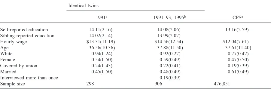
Table 1
Descriptive statistics: means and standard deviations
Identical twins
1991a 1991–93, 1995b CPSc
Self-reported education 14.11(2.16) 14.08(2.06) 13.16(2.59)
Sibling-reported education 14.02(2.14) 13.99(2.07) –
Hourly wage $13.31(11.19) $14.56(12.54) $12.04(7.61)
Age 36.56(10.36) 37.88(11.50) 37.61(11.40)
White 0.94(0.24) 0.92(0.27) 0.77(0.42)
Female 0.54(0.50) 0.59(0.49) 0.47(0.50)
Covered by union 0.24(0.43) 0.22(0.41) 0.19(0.39)
Married 0.45(0.50) 0.48(0.49) 0.61(0.49)
Interviewed more than once – 0.19(0.39) –
Sample size 298 906 476,851
aSource: Twinsburg Twins Survey, August 1991 (Ashenfelter & Krueger, 1994). bSource: Twinsburg Twins Survey, 1991–93, 1995.
cSource: The Current Population Survey (CPS) sample is drawn from the 1991–93 Outgoing Rotation Group files; the sample
includes workers age 18–65 with an hourly wage greater than $1.00 per hour in 1993 dollars and the means are weighted using the earnings weight.
teristics of my sample of twins with Ashenfelter & Krue-ger’s sample, and data from the Current Population Sur-vey (CPS) for the period 1991–93. The characteristics of the twins samples may differ from the CPS because the twins survey does not represent a random sample of twins or because twins do not share identical character-istics with the general population. It is apparent from Table 1 that the respondents in the twins samples are better educated and have a higher hourly wage than the general population. And, the twins samples contain rela-tively more white workers than the general population. All of these differences may arise from the way twins select themselves into the pool of Twins Festival attend-ers. The twins samples also contain relatively fewer mar-ried people than the general population. It is unclear what effect, if any, these differences would have on inferences one might draw from the samples of twins.4
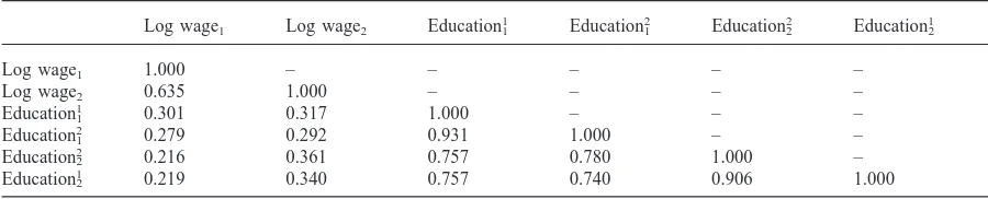
Further, the addition of three more years of surveys has changed the mean sample characteristics very little. The survey participants using the larger sample are a little older than Ashenfelter & Krueger’s sample, earn slightly more, and are more likely to be married and female. Table A1 of Appendix A shows the correlation matrix which allows for direct estimates of the extent of measurement error in (the cross-sectional) reported schooling in these data. Ashenfelter & Krueger estimate
4However, OLS estimates of log wage equations using the
twins sample and the CPS suggest only small differences between the primary characteristics of the two samples. In addition, the educational distribution in these data is extremely close to that reported in Lykken, Bouchard, McGue, & Tellegan (1990) from the Minnesota Twins Registry.
a reliability ratio5 for the schooling levels of between
0.92 and 0.88, implying that 8–12% of the measured variance in schooling is due to measurement error. The error in reported schooling in the larger sample is some-what lower with a reliability ratio of 0.93–0.91.
4. Empirical results
4.1. The basic results
Ashenfelter & Krueger’s basic OLS, generalized least squares (GLS),6
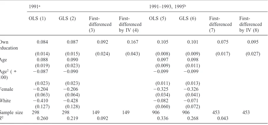
first-differenced, and IV estimates are reproduced in columns (1)–(4) of Table 2 along with similar regressions using the larger sample.7 Both the
OLS and GLS cross-sectional estimates of the return to schooling [in columns (5) and (6)] using the larger sam-ple are about 10%, slightly higher than those estimated by Ashenfelter & Krueger.
One can estimate the extent to which omitted ability is biasing the OLS estimate by comparing the schooling coefficient in column (3) to that in column (1) (for the bias before correcting for measurement error) or by com-paring the coefficients in columns (4) and (2) (for the
5The reliability ratio is the ratio of the variance in the true
level of schooling to the variance in the reported measure of schooling.
6The GLS estimates are the seemingly unrelated regression
method (Zellner, 1962). I use GLS to increase efficiency by exploiting cross-equation restrictions and to ensure correct com-putation of sampling errors.
Table 2
Ordinary least-squares (OLS), generalized least-squares (GLS), first-differenced, and instrumental variables (IV). Estimates of log wage equations for identical twins: Ashenfelter & Krueger’s results and those obtained with the larger sample
1991a 1991–1993, 1995b
OLS (1) GLS (2) First- First- OLS (5) GLS (6) First-
First-differenced differenced differenced differenced
(3) by IV (4) (7) by IV (8)
Own 0.084 0.087 0.092 0.167 0.105 0.101 0.075 0.095
education
(0.014) (0.015) (0.024) (0.043) (0.008) (0.009) (0.017) (0.027)
Age 0.088 0.090 0.097 0.098
(0.019) (0.023) (0.009) (0.011)
Age2(÷ 20.087 20.090 20.099 20.099
100)
(0.023) (0.023) (0.011) (0.013)
Female 20.204 20.206 20.325 20.326
(0.063) (0.064) (0.034) (0.041)
White 20.410 20.428 20.082 20.071
(0.127) (0.128) (0.060) (0.072)
Sample size 298 298 149 149 906 906 453 453
R2 0.260 0.219 0.092 0.336 0.268 0.043
Standard errors are in parentheses. All regressions include a constant. These regressions assume independent measurement errors.
aSource: Ashenfelter & Krueger (1994).
bSource: Twinsburg Twins Survey, 1991–93, 1995.
bias after correcting for measurement error). Ashen-felter & Krueger’s within-twin (or first-differenced) esti-mate of the return to schooling was higher than the com-parable cross-sectional estimate. This pattern is consistent with a downward bias in the OLS estimate due to an omitted family or ability effect (although the within-twin estimate is within a standard error of the cross-sectional estimate). In other words, they estimate that the correlation between omitted ability and school-ing may be slightly negative in cross-sectional analyses. An alternative explanation is offered by Griliches (1979) (and more recently Neumark (1999)) who shows that such a result is theoretically possible in the presence of upward ability bias in the OLS estimate if the upward ability bias is exacerbated in within-twin estimates. This would occur if the correlation between schooling and ability is larger within twins than across twins. This theoretical possibility is applicable to all twin and sibling studies, and a point to which I return in Section 4.3.
Analysis using the larger sample, however, suggests that Ashenfelter & Krueger’s result is an anomaly. Using all four years I estimate an upward bias in the OLS esti-mate of about 29%, before I correct for measurement error.8Further, when Ashenfelter & Krueger account for
8This result is consistent with most other within-twin (or
within-family) estimates of the return to schooling that also find an upward bias in the OLS estimate [see Altonji & Dunn (1996); Ashenfelter & Zimmerman (1997); Behrman, Rosenzweig, & Taubman (1994) for recent examples].
measurement error in this specification, their estimate of the return to schooling rises to a surprising 16.7%. Once measurement error is addressed using the larger sample, however, the estimated return to schooling rises to about 9.5%, and the estimated upward bias in the OLS estimate falls to 6%.9,10 Table 3 replicates the specifications in
9Given that the reliability ratio for the difference in twins’
schooling levels (assuming independent measurement errors) is about 0.62, as reported in Table A2 of Appendix A, the expected IV estimate is a return to schooling of 12.1% which is larger than the actual estimate of 9.5%. Note, however, that the actual estimate is within a standard error of the predicted estimate. The interested reader will also notice that in Table A2 of Appendix A the covariance betweenDS* andDLog Wage
does not equal the covariance betweenDS**andDLog Wage
(although they should since the twins are sorted randomly.) This apparent discrepancy is entirely due to sampling variability. I estimated these two covariances 2000 times randomly sorting the twins differently each time. The means of the two covari-ances are equal; the mean covariance is 0.192. In addition, the mean reliability ratio (for Table A2 of Appendix A) assuming independent measurement error is 0.613 and that allowing for correlated measurement error is 0.748; these are very close to the reported values.
10Ashenfelter & Krueger also control for ability by including
Table 3
OLS, GLS, first-differenced, and IV estimates of the log wage equations for identical twins: a direct comparison of Ashenfelter & Krueger’s results and those obtained using the larger samples
OLS(1) GLS(2) First-differenced(3) First-differenced by
IV(4)
Own education 0.112(0.010) 0.104(0.011) 0.047(0.022) 0.055(0.039)
Own education3 20.024(0.017) 20.010(0.019) 0.066(0.033) 0.083(0.054) interviewed in 1991
Interviewed in 1991 0.306(0.245) 0.098(0.265) – –
Age 0.098(0.009) 0.098(0.011) – –
Age2(÷100) 20.099(0.011) 20.099(0.013) – –
Female 20.326(0.034) 20.329(0.041) – –
White 20.081(0.061) 20.068(0.072) – –
Sample size 906 906 453 453
R2 0.338 0.269 0.051 –
Standard errors are in parentheses. All regressions include a constant. These regressions assume independent measurement errors. Source: Twinsburg Twins Survey, 1991–93, 1995.
Table 2 adding an interaction between whether the twins were interviewed in 1991 (and therefore in Ashen-felter & Krueger’s sample) in order to test for whether the discrepancies in the coefficients are statistically sig-nificant.11 While the first-differenced estimate that is
uncorrected for measurement error indicates that the dif-ference in the coefficients generated by the two samples is statistically significant at the 5% level, the preferred IV estimate of the difference has a P-value of 0.13. Given that similar survey instruments were employed on the same population using similar interview teams, the unexpected sign of the ability bias and the large magni-tudes in the return to schooling in Ashenfelter & Krueger are likely due to sampling variability.12
4.2. Independent and correlated measurement errors
The second innovation in Ashenfelter & Krueger’s paper is their ability to test for the presence of an individ-ual-specific component to the measurement error in
11I employ slightly different sample selection criteria than
Ashenfelter & Krueger which results in slightly different samples for 1991. However, if I restrict my sample to those interviewed in 1991, I get results qualitatively similar to those reported by Ashenfelter & Krueger.
12If I fully interact the model in column (1) with having
been interviewed in 1991, the P-value of the test of the joint significance of the interactions is 0.065. Much of the signifi-cance is driven by the interaction with whether the respondent is white, however, as the P-value rises to 0.14 when the interac-tion with race is excluded from the F-test. I have also interacted the difference in education in columns (7) and (8) with dummy variables indicating the year of the interview. The OLS esti-mates [that correspond to column (7)] indicate significant differ-ences between the years although the IV estimates do not. These results are available from the author on request.
schooling. If the individual-specific component of the measurement error is important, IV estimates assuming independent measurement errors will be inconsistent. Table 4 contains estimates that control for observable differences between twins while assuming both inde-pendent and correlated measurement errors.13The GLS
estimate that ignores the family effect is contained in the first column of Table 4. The cross-sectional estimate of the economic return to schooling, conditional on other covariates, is 11.1%. The fixed-effects estimate provided in column (2) of Table 4 falls to 8.9%. Column (3) in Table 4 usesDS9, the difference in the self-reported edu-cation levels, as the independent variable, andDS0, the difference in the sibling-reported estimates of the school-ing levels, as an instrumental variable forDS9. As Table 4 indicates, the IV estimate is about the same magnitude as the cross-sectional estimate in column (1).
The last two columns in Table 4 report the results of fitting Eq. (3) to the data using one twin’s report of the within-twin schooling difference as an instrument for the other twin’s report of the same difference. This strategy generates an estimate that is consistent in the presence of a person-specific component to the measurement error. Similar to the results in columns (2) and (3), the IV esti-mates that allow for correlated measurement errors are also close to the conventional cross-sectional estimates of the economic return to schooling. Although the indi-vidual-specific component to the error term should make the estimate assuming independent measurement errors larger than the estimate that relaxes this assumption, the
13In Table 4 I include other covariates to follow
Table 4
GLS, first-differenced, and IV estimates of the return to schooling for identical twins
Assuming independent measurement Assuming correlated measurement errorsb
errorsa
GLS(1) First-differenced(2) First-diff. by IV(3) First-differenced(4) First-diff. by IV(5)
Own education 0.111(0.009) 0.089(0.016) 0.110(0.027) 0.071(0.016) 0.119(0.021)
Age 0.091(0.011) – – – –
Age2()100) 20.104(0.013) – – – –
Female 20.261(0.041) – – – –
White 20.076(0.069) – – – –
Covered by a union 0.104(0.039) 0.087(0.050) 0.089(0.051) 0.085(0.051) 0.090(0.051) Married 0.039(0.035) 0.017(0.046) 0.017(0.046) 0.017(0.046) 0.015(0.047) Tenure (years) 0.020(0.002) 0.020(0.003) 0.020(0.003) 0.020(0.003) 0.021(0.003)
Sample size 890 445 445 445 445
R2 0.341 0.144 – 0.124 –
Standard errors are in parentheses. All regressions include a constant.
aThe difference in education is the difference between twin 1’s report of twin 1’s own education and twin 2’s report of twin 2’s
own education. The instrument used is the difference between twin 2’s report of twin 1’s education and twin 1’s report of twin 2’s education.
bThe difference in education is the difference between twin 1’s report of twin 1’s own education and twin 1’s report of twin 2’s
education; the instrument used is the difference between twin 2’s report of twin 1’s education and twin 2’s report of twin 2’s own education.
results in column (5) suggest a return to schooling of 12% compared to an estimate of 11% in column (3). This difference again highlights the importance of sampling error as the two estimates are well within a standard error of one another.14
Although the IV estimates suggest that the assumption of independence in the measurement errors is not econ-omically important, one can test the assumption more formally using a method of moments framework. The theoretical covariance matrix forDy,DS9,DS0,DS*, and
DS**implied by Eqs. (3)–(7) is reproduced in Table 5(a)
under the assumption that there is a person-specific component to the measurement error which is the frac-tion ‘rv’ of the total measurement error variance. (Thus,
rvis the correlation between the measurement errors in
the reports of schooling by one sibling.) Note that the
14This interpretation of the difference is reinforced by a
second (and underappreciated) source of variability in twin studies: the order of the twins is random. As a result, the first-differenced (‘fixed-effects’) estimates can vary depending on the order in which the data have been sorted. I have re-estimated the first-differenced estimates in Tables 2–4 2000 times ran-domly changing the order of the data each time. The estimates presented here are essentially at the mean of the estimates gen-erated; the only exceptions are that the mean estimates allowing for correlated measurement errors in Table 4 are 0.083 for col-umn (4) and 0.109 for colcol-umn (5). It is also worth noting that when I performed this same exercise using only the 1991 data, about 30% of the OLS within-twin estimates were lower than the cross-sectional estimate.
restriction rv 5 0 results in the theoretical covariance
matrix assuming independent measurement errors, i.e. the first three columns and rows of Table 5(a). Thus, the independent measurement error model is nested within the correlated measurement error model, and it is poss-ible to test the restriction. The empirical covariance matrix (that does not partial out the effects of other twin-specific characteristics) is presented in Table 5(b).
Table 6 contains generalized method of moments esti-mates (implemented using a maximum likelihood strat-egy with the statistical package LISREL) of the basic parameters set out in Tables 5(a) and (b). The estimates in columns (1)–(3) assume independent measurement errors. Because of the two measures of the difference in schooling levels, the parameters are over-identified. Separate estimates using each measure of the difference are in columns (1) and (2); estimates restricting these coefficients to be equal are in column (3). Again, the estimates of the return to schooling are smaller than those reported in Ashenfelter & Krueger. The restricted model [column (3)] suggests a return to schooling of 0.107 compared to an estimate of 0.162 reported in Ash-enfelter & Krueger. Thex2statistic of over-identifying
restrictions, presented at the bottom of the table, indi-cates that the restrictions are not rejected.15I present the
15These estimates are not fully efficient because not all of
Table 5
(a)Theoretical covariance matrix; (b) empirical covariance matrix
(a) Dy DS9 DS0 DS* DS**
Dy b2s2
DS1 bs2DS bsD2S bs2DS bs2DS
s2De
DS9 – s2
DS12s2n9 s2DS22rnsn9sn0 sD2S1s2n92rnsn9sn0 s2DS1s2n92rnsn9sn0
DS0 – – s2
DS12s2n0 s2DS1s2n02rnsn9sn0 s2DS1s2n02rnsn9sn0
DS* – – – s2
DS1s2n91s2n02rnsn9sn0 s2DS
DS** – – – – s2
DS1s2n91s2n02rnsn9sn0
(b)
Dy 0.279 0.167 0.129 0.129 0.167
DS9 – 2.060 1.339 1.723 1.676
DS0 – – 2.286 1.894 1.731
DS* – – – 2.095 1.521
DS** – – – – 1.886
There are 445 observations.
Table 6
Generalized method of moments estimates
Independent errors Correlated errors
Unrestricted estimates Restricted estimates Restricted estimates
Parameter (1) (2) (3) (4) (5)
b 0.096(0.028) 0.125(0.027) 0.113(0.024) 0.105(0.023) 0.099(0.021)
s2
DS 1.339(0.121) 1.339(0.121) 1.342(0.121) 1.441(0.119) 1.524(0.119)
s2De 0.267(0.018) 0.258(0.018) 0.262(0.018) 0.264(0.018) 0.265(0.018)
s2Dn9 0.721(0.094) 0.721(0.094) 0.700(0.092) – –
s2Dn0 0.947(0.103) 0.947(0.103) 0.967(0.102) – –
s2Dn9 – – – 0.275(0.037) 0.260(0.042)
s2Dn0 – – – 0.381(0.040) 0.394(0.045)
rn – – – – 0.289(0.047)
x2(dof) (P-value) NA NA 1.359(1)(0.244) 45.781 (7)(0.000) 11.158 (6)(0.084)
Estimated asymptotic standard errors are in parentheses. In column (4) rv is constrained to equal zero. ‘dof’ are the degrees of
freedom. These are generalized method of moments estimates assuming that the errors are normally distributed.
correlated measurement error model that restrictsrv to
zero in column (4) and that allowsrvto vary in column
(5). The economic return to schooling assuming no cor-relation between the errors is 0.105 and falls to 0.099 when the errors are allowed to be correlated. The esti-mate ofrvsuggests a fair degree of positive correlation
between the two error terms that is statistically signifi-cant,16although the correlation is smaller in magnitude
than that reported by Ashenfelter & Krueger. The results in Table 6 provide clear evidence of an important person-specific component to the measurement error in school-ing levels.
16In addition, a likelihood ratio test between the two models
rejects the model that restricts the correlation to be zero.
4.3. Within-twin vs cross-sectional estimates of the return to schooling
As originally highlighted by Griliches (1979), a poten-tially important issue with twin (and within-sibling) estimates of the return to schooling is whether the resulting estimates are actually less (upward) biased than cross-sectional estimates. If the ratio of the within-twin variance in ability to the within-within-twin variance in schooling is greater than the ratio of the cross-sectional variance in ability to the cross-sectional variance in schooling, then within-twin estimates of the return to schooling may actually be more upward biased than cross-sectional estimates.
(1998) provide (indirect) evidence that cross-sectional estimates of the return to schooling likely contain more upward ability bias than within-twin estimates. For example, approximately 60% of the cross-sectional vari-ance in schooling is between families (once corrected for measurement error), and between family measures of schooling are highly correlated with observables such as marital status, union status, job tenure, and spouse’s edu-cation, whereas the within-twin measures of schooling are not.
In addition, in all cases presented here, the cross-sec-tional estimates are greater than the within-twin esti-mates, whether or not the within-twin estimates are cor-rected for measurement error. Therefore, to the extent that omitted ability is upward biasing the within-twin estimates, it is more severe in the cross-sectional esti-mates.
A final point made by Neumark (1999) is that because the OLS within-twin estimates of the return to schooling suffer from both downward and upward biases (due to measurement error and ability biases), whereas the IV within-twin estimates only suffer from upward biases (due to ability bias), the OLS within-twin estimate of the return to schooling may most accurately reflect the ‘true’ return to schooling. This situation would exist if the within-twin ability bias were large enough to off-set the (relatively large) measurement error bias. This is a theor-etical possibility that requires an estimate of the magni-tude of the potential ability bias in twins analyses. While the magnitude of this bias is currently unknown, the upward ability bias in cross-sectional estimates likely provides an upper-bound. Given that recent IV estimates of the return to schooling employing other identifying strategies suggest little ability bias in cross-sectional esti-mates [e.g. Angrist & Krueger (1991); Card (1993); Kane & Rouse (1993)], the overall evidence likely favors the measurement error corrected within-twin estimates.
5. Conclusion
The results in this paper using additional data on twins indicate that each year of schooling increases earnings by
Table A1
Cross-sectional correlation matrix for identical twins
Log wage1 Log wage2 Education11 Education21 Education22 Education12
Log wage1 1.000 – – – – –
2 0.216 0.361 0.757 0.780 1.000 –
Education1
2 0.219 0.340 0.757 0.740 0.906 1.000
‘Log Wagek’ is twin ‘k’s’ report of his/her own wage, ‘Educationkj’ is twin ‘j’s’ report of twin ‘k’s’ education.
about 10%, smaller than Ashenfelter & Krueger’s final estimate of 13%. More importantly, unlike the results reported by Ashenfelter & Krueger, the larger sample of identical twins indicates that schooling levels are posi-tively correlated with ability in cross-sectional analyses. Finally, a model assuming no individual-specific compo-nent to the measurement error in schooling levels is rejected by the data.
Acknowledgements
I thank Michael Boozer, Alan Krueger, and Douglas Staiger for useful conversations, Lisa Barrow, Casundra Anne Cliatt, Lasagne Anne Cliatt, Eugena Estes, Kevin Hallock, Dean Hyslop, Jon Orszag, Michael Quinn, Lara Shore-Sheppard, and Cedric Tille for excellent assistance with the survey, John Abowd for access to LISREL, and three anonymous referees for helpful comments. This paper has been supported by the Mellon Foundation and The National Academy of Education and the NAE Spen-cer Postdoctoral Fellowship Program.
Appendix A
Table A2
Within-twin correlation matrix for identical twins
DLog wage DS9 DS0 DS* DS**
DLog wage 1.000 – – – –
DS9 0.220 1.000 – – –
DS0 0.162 0.617 1.000 – –
DS* 0.169 0.829 0.865 1.000 –
DS** 0.230 0.850 0.834 0.765 1.000
Table A3
GLS, first-differenced, and IV estimates of the return to schooling for identical twins excluding the 1991 survey
Assuming independent measurement Assuming correlated measurement errorsb
errorsa
GLS(1) First-differenced(2) First-diff. by IV(3) First-differenced(4) First-differenced by IV(5)
Own education 0.115(0.010) 0.069(0.022) 0.076(0.039) 0.040(0.021) 0.104(0.030)
Age 0.089(0.013) – – – –
Age2(÷100) 20.098(0.016) – – – –
Female 20.319(0.049) – – – –
White 20.001(0.075) – – – –
Covered by a union 0.080(0.047) 0.062(0.061) 0.061(0.061) 0.065(0.062) 0.066(0.063) Married 0.027(0.041) 20.029(0.055) 20.029(0.055) 20.029(0.056) 20.032(0.057) Tenure (years) 0.019(0.003) 0.015(0.003) 0.015(0.004) 0.015(0.004) 0.016(0.004)
Sample size 588 294 294 294 294
R2 0.375 0.085 – 0.065 –
Standard errors are in parentheses. All regressions include a constant.
aThe difference in education is the difference between twin 1’s report of twin 1’s own education and twin 2’s report of twin 2’s
own education. The instrument used is the difference between twin 2’s report of twin 1’s education and twin 1’s report of twin 2’s education.
bThe difference in education is the difference between twin 1’s report of twin 1’s own education and twin 1’s report of twin 2’s
education; the instrument used is the difference between twin 2’s report of twin 1’s education and twin 2’s report of twin 2’s own education.
References
Altonji, J., & Dunn, T. (1996). The effects of family character-istics on the return to education. Review of Economics and Statistics, 78, 692–704.
Angrist, J.D., & Krueger, A. (1991). Does compulsory school affect schooling and earnings? Quarterly Journal of Eco-nomics, 106, 979–1014.
Ashenfelter, O., & Krueger, A. (1994). Estimating the returns to schooling using a new sample of twins. American Economic Review, 84, 1157–1173.
Ashenfelter, O., & Rouse, C. (1998). Income, schooling, and ability: Evidence from a new sample of identical twins. Quarterly Journal of Economics, 113, 253–284.
Ashenfelter, O., & Zimmerman, D.J. (1997). Estimates of the return to schooling from sibling data: Fathers, sons, and bro-thers. Review of Economics and Statistics, 79, 1–9. Behrman, J.R., Hrubec, Z., Taubman, P., & Wales, T.J. (1980).
Socioeconomic success: A study of the effects of genetic endowments, family environment, and schooling. Amster-dam: North-Holland.
Behrman, J.R., Rosenzweig, M.R., & Taubman, P. (1994). Endowments and the allocation of schooling in the family
and in the marriage market: the twins experiment. Journal of Political Economy, 102, 1131–1174.
Card, D. (1993). Using geographic variation in college proxim-ity to estimate the return to schooling. National Bureau of Economic Research Working Paper No. 4482, October. Griliches, Z. (1977). Estimating the returns to schooling: some
econometric problems. Econometrica, 45, 1–22.
Griliches, Z. (1979). Sibling models and data in economics: beginnings of a survey. Journal of Political Economy, 87, S37–S64.
Kane, T.J., & Rouse, C.E. (1993). Labor market returns to two-and four-year college: Is a credit a credit two-and do degrees matter? Princeton University Industrial Relations Section Working Paper No. 311.
Lykken, D.T., Bouchard, T.J., McGue, M., & Tellegan, A. (1990). The Minnesota twin family registry: Some initial findings. Acta Genetica et Medica Gemellologia, 39, 35–70. Neumark, D. (1999). Biases in twin estimates of the return to schooling: A note on recent research. Economics of Edu-cation Review, 18(2), 0–00.