Minimizing the expected total value of shortages for
a population of items subject to practical restrictions
on the reorder points
Ilkyeong Moon
!
,
*
, Edward A. Silver
"
!Department of Industrial Engineering, Pusan National University, Pusan 609-735, South Korea
"Faculty of Management, The University of Calgary, Calgary, Alb., Canada
Received 8 November 1999; accepted 7 April 2000 Abstract
We address a problem of setting reorder points (expressed as time supplies) of a population of items, subject to a restricted set of possible time supplies as well as a budget on the total amount of safety stocks, both important practical constraints. We provide a branch-and-bound algorithm for obtaining the optimal solution. In addition, a simple and e$cient heuristic algorithm has been developed. Computational experiments show that the performance of the heuristic is excellent based on a set of realistic examples. However, the typical set of possible time supplies may signi"cantly degrade performance compared with the situation where a continuum of choices are possible. ( 2001 Elsevier Science B.V. All rights reserved.
Keywords: Inventory; Safety stock; Lower bound; Branch and bound; Heuristic
1. Introduction
Managers are concerned with the e!ective use of limited resources. An example is the allocation of a speci"c budget among the safety stocks of a popu-lation of items, each of which is controlled by a continuous review, order point and order quan-tity system. One possible criterion is the minimiz-ation of an aggregate measure of disservice, such as the expected total value of units short per year (ETVSPY). The case where there is no restriction,
*Corresponding author. Tel.:#82-51-510-2451; fax:# 82-51-512-7603.
E-mail address:[email protected] (I. Moon).
other than the budget constraint, on the choice of safety stocks (or reorder points) has been treated in the literature [1]. In fact, by varying the levels of the available budget, one can trace out a whole exchange curve which shows the best that one can do on the service measure as the budget is varied (see, for example, [2] or [3]). However, these results hinge upon continuous possible values of the deci-sion variables (the reorder points or, equivalently, the safety stocks); but, in practice, managers often prefer to restrict the decision variables to a set of easily understood and implementable discrete values, e.g. the reorder point, expressed as a time supply, which is restricted to one of the following values: 1 week, 2 weeks, 1 month, 2 months, 3 months, 6 months or 1 year.
This paper addresses how to deal with the above-constrained problem in a pragmatic fashion. Speci"cally, we treat the case where there is a set of time supplies, one of which must be used for each of a population of items. There is a speci"ed upper limit on the total value of safety stock to be used and we wish to choose the time supply reorder points of the population of items, subject to a dis-crete set of options and the aggregate constraint, so as to minimize the expected total values of the units short per year.
In the next section, we introduce the notation and mathematically formulate the problem, includ-ing obtaininclud-ing a useful lower bound. This is followed by the speci"cation of an optimal solution proced-ure using a branch-and-bound algorithm. The as-sociated computational e!ort required increases substantially with the number of items. Perhaps more important, branch and bound is a very di$ -cult concept to explain to practitioners. Therefore, we subsequently present a heuristic approach that overcomes both of these drawbacks. Moreover, we present results of computational experiments that show that very little degradation in the objective function value results from using the heuristic in-stead of the optimal solution. However, the perfor-mance of the optimal solution is markedly a!ected by the discrete choice of the time supplies, parti-cularly if the set is fairly sparse as would likely be the case in practice.
2. Problem formulation and a lower bound
The notation to be used is as follows:
n number of items
D
i the demand rate of itemi"1, i, in units/unit time, 2,n
v
i the unit variable cost of itemunits/unit,i"1, i, in monetary 2,n
x(i the mean lead time demand of item i,
i"1,2,n p
i the standard deviation of lead time demand ofitemi,i"1, 2,n
Q
i the predetermined order quantity of itemi"1, i, 2,n
> total budget for safety stocks
t
i the reorder point of itemsupply),i"1, i(expressed as a time 2,n
¹ the discrete set of possible time supplies
m number of possible discrete reorder time sup-plies, and
¹
j thej"1,jth possible reorder time supply, 2,m
There are many di!erent methods of selecting safety stocks (or reorder points) in control systems under probabilistic demand. In this paper, we use the criterion of minimization of expected total value short per year subject to a speci"ed total safety stock. The assumptions are exactly the same as for the classical multi-item (s,Q) inventory model with a budget constraint on the total safety stock (see [3]) except that we add the important practical consideration that the time supplies are limited to a discrete set ¹. Without loss of generality, we assume that the items are numbered such that
D
1v1*D2v2*2*Dnvn. We assume that lead
time demand follows a normal distribution. De"ne
G u(k) as
G u(k)"
P
=
k
(u!k) 1
J2pexp(!u2/2) du,
which measures the expected number of units of demand in excess of supply in each replenishment cycle.
Then our problem can be represented as follows:
(ETVSPY)
Min ETVSPY"+n i/1
D i Q i
p
iviGu
A
Diti!x(i
p
i
B
s.t.
n
+
i/1 D
iviti)>@, (1)
t
i3M¹1,¹2,2,¹mN, ∀i, (2)
where
>@">#+n i/1
x(iv i.
We derive a lower bound on (ETVSPY) for two reasons. First, the lower bound is the optimal value of the objective function when thet
i's are not
Table 1
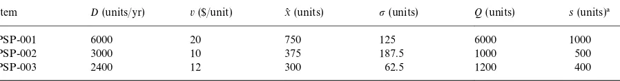
Data for the 3 item example
Item D(units/yr) v($/unit) x( (units) p(units) Q(units) s(units)!
PSP-001 6000 20 750 125 6000 1000
PSP-002 3000 10 375 187.5 1000 500
PSP-003 2400 12 300 62.5 1200 400
!s: reorder point.
in the expected total value short per year) caused by the introduction of the pragmatic constraint of restricting thet
i's to the discrete set¹. Second the
lower bound solution will be used as a starting point in our heuristic approach.
If we relax constraint (2), we obtain the following relaxed version of (ETVSPY):
(LB) Min ETVSPY"+n
Note that constraint (3) holds as a strict equality. Observe that the objective function is a convex decreasing function oft
i, ∀i. Note thatj'0 is an
optimal Lagrange multiplier.
If we can "nd a Karush}Kuhn}Tucker (KKT) solution, it will be a global minimum due to the fact that the objective function is convex and the set of feasible solutions is a convex set and is non-empty if >@'0. The Lagrangian function is as follows:
¸(t
The Karush}Kuhn}Tucker conditions require (see also [3])
is the right-hand tail of the unit normal distribution and represents the probability of a stockout during a replenishment lead time. Simplifying, we obtain
j"Di
Note that Eq. (4) implies that the expected number of cycles per year during which stockouts occur is the same for all items and that this value equals the value of the Lagrangian multiplier. We can use the following line search algorithm to "nd a solution that satis"es (4) and (5).
ciated optimal solution for (LB), sayt0@
i s.
If+ni/1D
iviti(>@, decreasejand go to Step 2.
If+ni/1D
iviti'>@, increasejand go to Step 2.
We now illustrate the above algorithm using an example found in [3], which is reproduced in Table 1. The three items are produced and stocked by a company. It is not uncommon for organiza-tions to use the following type of rule for setting reorder points for a broad range of items: reorder when the inventory position has dropped to a
spe-ci"c time supply. We assume that the current
reor-der points of the company are each based on a two-month time supply (that is,D/6).
Assuming normally distributed lead time de-mand, the safety stock and ETVSPY using the current policy are as listed under the title of&equal time supply'in Table 2. If we use the algorithm to
Table 2
Results for the 3 item example
Item no. Equal time supply Optimal
SS! ETVSPY SS! ETVSPY
1 $5000 $21 $2972 $143.4
2 $1250 $845 $3302 $88.5
3 $1200 $35 $1175 $37.7
Total $7450 $901/yr $7450 $269.6/yr
!SS: safety stock, ETVSPY: expected total value short per year.
which is equivalent to the optimal solution under continuous possible time supplies, we can achieve 70% savings compared to the strategy based on equal probabilities of stockout per cycle.
3. Branch-and-bound algorithm for optimal solution
Because of the discrete nature of the ¹ j's we
develop a branch-and-bound scheme to solve (ETVSPY). Since we use the heuristic (which has been presented in Section 4) as an upper bound and its performance is quite good (which will be demon-strated later), we believe that most branches will be fathomed in early stages, especially branches with small t values. In addition, the budget constraint also plays a role in eliminating many branches in early stages, especially branches with largetvalues. Nevertheless, we conjecture that (ETVSPY) is an NP-hard problem [4], hence there is a need, from a computational standpoint, for a heuristic solution procedure for large instances of the problem. The problem is a knapsack like problem and hence inherits its computational complexity from this problem.
The branch-and-bound algorithm is outlined be-low.
Step 1: Start from item 1 (the item with the largestDvvalue).
(i)Branching: Produce m branches in which each branch corresponds to one value from¹.
(ii)Bounding: We use the value of the heuristic as an initial upper bound (VAL
U). If we "nd a better solution during the branch-and-bound al-gorithm, it will be a new upper bound.
(iii)Fathoming: A branch will be fathomed if either of the following condition is satis"ed.
(a) If thet
1 value and the smallest assignment of t
2totnspend more than the budget, the branch will
be fathomed. That is, If
D
1v1t1# n
+
i/2 D
ivi¹1'>@, the branch is fathomed.
(b) If the t
1 value and the largest assignment of t
2 to tn give an objective value larger than
the current upper bound, the branch is fathomed. That is,
If
D 1 Q
1 p1v
1Gu
A
D1t1!x(1
p1
B
#+n i/2
D i Q i
p
iviGu
A
Di¹m!x(i
p
i
B
'VAL U,
the branch will be fathomed.
Step 2: (i)Branching:
Producembranches for each of the branches not fathomed in Step 1.
(ii)Bounding: same as before. (iii)Fathoming:
(a) If thet
1andt2values and the smallest assign-ment oft
3 totn spend more than the budget, the
branch is fathomed. That is, If
2
+
i/1 D
iviti# n
+
i/3 D
ivi¹1'>@,
the branch will be fathomed. (b) If thet
1andt2values and the largest assign-ment of t
3 to tn give an objective value larger
fathomed. That is, the branch will be fathomed.
Repeat this procedure until all the branches are either searched or fathomed.
Note: We could have developed a dynamic pro-gramming formulation for this problem similar to that of the knapsack problem. However, the size of the problem would become enormous due to the noninteger nature of theDvtvalues.
The branch-and-bound algorithm has been coded using GAUSS [5], and it has been run on an IBM Pentium II PC with 266 MHz clock speed. A depth-"rst-search method has been used to avoid a memory problem.
4. Heuristic algorithm
We develop a heuristic algorithm for (ETVSPY) since, as mentioned earlier, it would take much time to solve the branch-and-bound algorithm if n be-comes quite large. Moreover, the heuristic solution is much easier for a practitioner to understand than is a branch-and-bound algorithm. Note that we can obtain an upper bound directly from the lower bound solution of thet
i's. That is, if we round the t0
i's down to the nearest¹j's, we obtain an upper
bound (a feasible solution) immediately. The heu-ristic algorithm is based on starting with the lower bound (infeasible) solution and then using a mar-ginal (or greedy) allocation algorithm [6] to change the solution. At each step of the algorithm, we"nd the item that least increases the objective value per unit decrease of the stock investment. This item's reorder point is then reduced to the next lower value in¹. This is continued until a feasible solu-tion is obtained. Any remaining capacity is"lled in a reverse greedy fashion.
Step 1: Solve the lower bound problem. Lett0 i be
the lower bound solution fort i.
Step 2: Suppose ¹
ri(t0i(¹ri`1 (if t0i"¹ri or
¹
ri`1, we just leave t0i as it is). Round up all t0i's
obtained in solving (LB) to the nearest ¹ j (this
solution will always be infeasible unless
t0
i3¹"M¹1,2,¹mN∀i since the t0i's satisfy
con-straint (1) as an equality). Let the current value of
t
i be¹li.
Step 3: Choose the itemisuch that
G
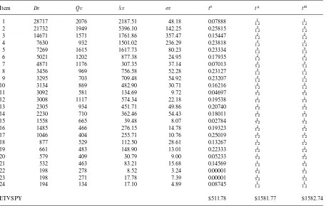
pNumerical example. We solved a randomly gener-ated 24 item problem (The method of generation will be explained in Section 5). The data for this problem are in Table 3.
Table 3
Data for the 24 item example and lower bound, optimal, and heuristic solutions!
Item Dv Qv x(v pv t0 tH tH
1 28717 2076 2187.51 48.18 0.07888 121 121
2 21732 1949 5396.10 142.25 0.25815 123 123
3 14671 1571 1761.86 357.47 0.15447 122 122
4 7630 932 1501.02 236.29 0.23818 123 123
5 7269 1615 1617.73 80.23 0.23334 123 123
6 5021 1202 877.38 24.95 0.17935 122 122
7 4871 1176 307.35 37.14 0.07013 523 523
8 3456 969 756.58 52.28 0.23127 123 123
9 3295 703 709.48 54.92 0.23207 123 123
10 3134 869 482.90 30.71 0.16216 122 122
11 3092 581 134.69 9.72 0.04697 523 523
12 3008 1117 574.34 22.18 0.19538 122 122
13 2305 934 451.71 49.86 0.20740 122 122
14 2230 710 362.46 54.43 0.18011 122 122
15 1558 665 39.48 8.07 0.02784 521 521
16 1485 466 276.15 14.78 0.19323 122 122
17 1046 404 255.71 10.76 0.25019 123 123
18 877 529 112.50 28.61 0.13267 121 121
19 661 483 148.90 13.01 0.22333 122 122
20 579 409 30.79 9.00 0.05233 521 522
21 532 463 83.21 15.68 0.14569 121 523
22 198 278 8.52 3.24 0.00001 521 521
23 198 271 17.78 7.39 0.00001 521 521
24 194 134 17.10 4.89 0.08745 121 121
ETVSPY $511.78 $1581.77 $1582.74
!t0: lower bound solution,tH: optimal solution,tH: heuristic solution.
tH6"2
12, tH7" 3 52, tH8"
3 12, tH9"
3
12, tH10" 2 12,
tH11"3
52, tH12" 2 12,tH13"
2
12, tH14" 2
12, tH15" 1 52,
tH16"2
12, tH17" 3
12, tH18" 1 12,tH19"
2
12, tH20" 1 52,
tH21"1
12, tH22" 1
52, tH23" 1
52, tH24" 1 12.
The optimal objective value is 1581.77.
We also solved the same 24 item example, but this time using the heuristic algorithm.
Step 1: First, we compute the lower bound solu-tion using the line search algorithm in Secsolu-tion 2.
The lower bound solution is as follows:
t01"0.07888, t02"0.25815, t03"0.15447,
t04"0.23818, t05"0.23334, t06"0.17935,
t07"0.07013, t08"0.23127, t09"0.23207,
t010"0.16216, t011"0.04697, t012"0.19538,
t013"0.20740, t014"0.18011, t015"0.02784,
t016"0.19323, t017"0.25019, t018"0.13267,
t019"0.22333, t020"0.05233, t021"0.14569,
t022"0.00001, t023"0.00001, t024"0.08745.
The value of the lower bound is 511.78.
Step 2: Round up the t0
i's to the nearest ¹j's,
objective value of the infeasible solution is 104.17.
Steps 3 and 4: We compute the priority ratios of the reduction of the t values dynamically using Eq. (6). The priority order of the reduction of the
tvalues is as follows:
17, 24, 2, 14, 6, 16, 12, 15, 18, 20, 13, 21, 19,
7, 24, 21.
It means that we"rst reducet
17from124 to123, and check whether +ni/1D
iviti)>@. We iterate this
procedure until we satisfy +ni/1D
iviti)19 562.
This"nally occurs when we decreaset
21 from121 to 3
52. Since+ni/1Diviti"19 554(19 562, we move to
Step 5.
Step 5: Since we have $8 remaining, we want to use them up if possible. We compute the priority ratios of the increase of the t values dynamically using Eq. (7). The priority order of the increase of thetvalues is as follows:
21, 24, 7, 19, 13, 20, 18, 15, 12, 16, 23, 22, 6, 2.
Since we cannot increase t
21 from 523 to 121, we increaset
24from523 to121. Since, we have only$3.76 remaining budget, which cannot be used to increase any of thet
i's, after this assignment, we stop here.
Note that the priority order of the increases in the
tvalues is not necessarily in the exact reverse order to that of Step 3 reduction of the tvalues.
The heuristic solution is as follows (we put the lower bound solution, an optimal solution, and the heuristic solution together in Table 3 for easier
comparison):
The objective value of the heuristic solution be-comes 1582.74. Note that this solution is di!erent from the optimal solution in two elements. Speci" -cally,t
20"522, andt21"523, compared totH20"521 andtH21"1
12. The ratio of the objective value of the heuristic solution to that of the optimal solution is 1.0006, an extremely small cost penalty.
5. Computational studies
First, we have solved a 48 item problem of Brown [2] where it was necessary to generate the
x( andpvalues. We varied the size of the¹set to see how the heuristic performs as the problem becomes similar to the continuous one. The excellent perfor-mance of the heuristic, at least in a limiting sense, can be con"rmed as follows. The larger the size of the ¹ set, the smaller the ratio VAL
H/VALLB, where VAL
Hand VALLBare the objective function value obtained by the heuristic and the lower bound procedure, respectively. Note that we could
not"nd an optimal solution using the
branch-and-bound algorithm since the computational burden becomes enormous (Table 4).
Table 4
Performance of the heuristic by varying the size of the set of time supplies
¹set VAL
H/VALLB
¹"M521,522,523,121,122,123,124,125,126N 44.8036
¹"M521,522,523,2,52
52N 1.9315
¹"M1
52,522,523,2,5252NXM3651,3652 ,3654 ,3658,2,128365,256365N 1.8449 ¹"M 1
365,3652,3653 ,2,365365N 1.0355
¹"M 1
1000,10002 ,10003 ,2,10001000N 1.0026
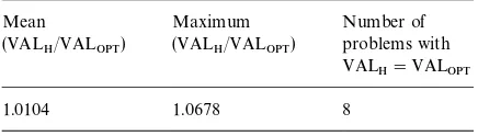
Table 5
Computational results for randomly generated problems Mean
(VAL
H/VALOPT)
Maximum (VAL
H/VALOPT)
Number of problems with VAL
H"VALOPT
1.0104 1.0678 8
be denoted by x, thenxfollows the distribution
f(x)" 1
bxJ2pexp
C
!(lnx!a)2
2b2
D
, 0(x(R,where a and b are the mean and the standard deviation of the underlying normal distribution. It can be shown that the mean value of the lognormal distribution is given by
E(x)"exp
C
a#b2 2D
and the coe$cient of variation (a measure of the relative dispersion) of the lognormal distribution is a monotonically increasing function of onlyb. Ac-cording to Herron [8], typically the inventories of merchants (wholesalers, retailers, etc.) have b's in the range of 0.8}2.0; industrial producers in the range 2}3; and highly sophisticated hardware sup-pliers (who are subject to rapid technological in-novations) haveb's in the 3}4 range. Thus, we set the parameter values within these ranges. We have solved 25 randomly generated problems. Since the objective function for our problem can be trans-formed as follows, we only need to generaten,D
ivi,
piv
i, Qivi, ¸i and >parameters. We can then
re-write ETVSPY as
ETVSPY"+n i/1
D ivi Q
ivi
(p
ivi)Gu
A
Diviti!x(ivi
p
ivi
B
.
We have generated those parameter values as fol-lows:
n&Uniform(15, 30), ¸&Uniform(1, 13)weeks,
Dv&LN(7.55, 1.52),
pv"J¸c 1
A
Dv
52
B
c2
where c
1&Uniform(0.5, 1) and c
2&Uniform(0.5, 1). Since Q
ivi"J2AiDivi/ri, we need to generate Aandrin order to generateQv.
A&Uniform(10, 50), r"0.24/year,
>&Uniform(1, 2.5)]+n
i/1 p
ivi.
The computational results for the 25 randomly generated problems have been summarized in Table 5. Here VAL
OPT represents the optimal ob-jective value. The performance of the heuristic is reasonable. The few problems with the higher penalties (still only 5}7%) have the following com-mon characteristic. In Step 3 of the heuristic, the budget reduction associated with the last item, whoset
i was lowered, left a relatively large unused
budget (i.e. undershoot of the constraint). Then in Step 5 manyt
ivalues had to be increased, a process
which apparently does not get as close to the opti-mal solution as does the main part of the Heuristic (Step 3) which begins with an infeasible solution and reducest
i's (this is consistent with the"ndings
di!erent heuristic, starting from roundingdownthe lower bound solution to the nearest ¹
j's. Speci"
-cally, this reverse type of heuristic did not work as well as the one described in this paper).
We did not test problems having more than 30 items because of the computational burden asso-ciated with the branch and bound algorithm for this size. However, we developed an approximate dynamic program which can be used to solve large size problems. The idea is to divide both sides of the budget constraint by a constant to reduce the number of states. Clearly, it does not necessarily produce an optimal solution. We have tested 25 randomly generated problems with
n values between 50 to 100. Interestingly, our heuristic outperformed the approximate dynamic program.
6. Conclusions
In this paper we have analyzed a problem of setting reorder points (or safety stocks) of a popula-tion of items, subject to a restricted set of possible values (expressed as time supplies) as well as a limit on the total value of the safety stock. A branch-and-bound formulation for obtaining the optimal solution has been presented. In addition, a much simpler heuristic solution procedure has been shown to provide excellent results on a set of realis-tic examples. However, the incorporation of the pragmatic constraint of a restricted set of time supplies tends to severely deteriorate the perfor-mance (much higher ETVSPY for a given safety stock budget) compared with the unrestricted case. This is particularly true when the set of possible time supplies is fairly sparse, particularly at the lower end, which is likely to be the case in practice. Thus, the message for practitioners is clear, namely that management's desire for an easily understood and implementable reorder point policy may come with a high associated cost in terms of degradation of service. This contrasts with our earlier"ndings [9] for a similar problem of selecting order quantit-ies subject to a prescribed maximum number of replenishments per year. A possible way of at least partially improving the performance for a speci"ed total number of possible time supplies would be to
choose them so that they are more tightly packed at the lower end, such as by the so-called powers-of-two approach [10]. Speci"cally, one would choose the smallest time supply at a conve-nient value, such as 1 day, then have the higher ones at powers of two, i.e. 2, 4, 8, 16, etc., times this value. In Table 4, we can see that the performance has been slightly improved by adopting this ap-proach.
Acknowledgements
The authors are grateful to Professor Inchan Choi and Dr. Sang-Jin Choi for the suggestions on the branch-and-bounding coding and two anony-mous referees for their valuable comments. The research leading to this paper was partially carried out while Edward Silver held a Visiting Erskine Fellowship in the Department of Management at the University of Canterbury, New Zealand and while Ilkyeong Moon held a visiting position in the Faculty of Management at the University of Cal-gary during a sabbatical leave. The research has been supported by the Brain Korea (BK) 21 project in the year 1999 sponsored by the Ministry of Education in Korea, by the Natural Sciences and Engineering Research Council of Canada under Grant A1485, and by the Carma Chair at the Uni-versity of Calgary.
References
[1] G. Gerson, R. Brown, Decision rules for equal shortage policies, Naval Research Logistics Quarterly 3 (1970) 351}358.
[2] R. Brown, Decision Rules for Inventory Management, Holt, Rinehart and Winston, New York, 1967.
[3] E. Silver, D. Pyke, R. Peterson, Inventory Management and Production Planning and Scheduling, 3rd Edition, Wiley, New York, 1998.
[4] M. Garey, D. Johnson, Computers and Intractability: A Guide to the Theory of NP-Completeness, Freeman, San Francisco, 1979.
[5] Aptech Systems, GAUSS System Version 3.2.32, Aptech Systems, Inc., Maple Valley, WA, 1997.
[7] M. Starr, D. Miller, Inventory Control: Theory and Prac-tice, Prentice-Hall, Englewood Cli!s, NJ, 1962.
[8] D. Herron, Industrial engineering applications of ABC curves, AIIE Transactions 8 (1976) 210}218.
[9] E. Silver, I. Moon, A fast heuristic for minimizing total average cycle stock for a population of items subject to
practical constraints, Journal of the Operational Research Society 50 (1999) 789}796.